Taguchi-Based and Intelligent Optimisation of a
Multi-Response Process Using Historical Data
Šibalija, T. ‒ Majstorović, V. ‒ Soković, M. Tatjana Šibalija1,* ‒ Vidosav Majstorović1 ‒ Mirko Soković2 1 University of Belgrade, Faculty of Mechanical Engineering, Serbia 2 University of Ljubljana, Faculty of Mechanical Engineering, Slovenia
Optimisation of manufacturing processes is typically performed by utilising mathematical process models or designed experiments. However, such approaches could not be used in the case when explicit quality function is unknown and when actual experimentation would be expensive and time-consuming.
The paper presents an approach to optimisation of manufacturing processes with multiple potentially correlated responses, using historical process data. The integrated approach is consisted from two methods: the first relays on Taguchi’s quality loss function and multivariate statistical methods, the second method is based on the first one and employs artificial neural networks and a genetic algorithm to ensure global optimal settings of a critical parameters found in a continual space of solutions.
The case study of a multi-response process with correlated responses was used to illustrate the effective application of the proposed approach, where historical data collected during normal production and stored in a control charts were used for process optimisation.
© 2011 Journal of Mechanical Engineering. All rights reserved.
Keywords: optimisation, historical data, Taguchi method, neural networks, genetic algorithm
0 INTRODUCTION
Process optimisation is typically performed by analysing the process responses obtained from designed experiments, carried out on the actual manufacturing process. However, conducting experiments on the actual process tends to cause distruption in the plant and may be uneconomic. The possibility to use process historical data (i.e. from the control charts) has not been explored videly in the literature. There are few studies that used historical data for optimisation, but they discuss only single-response problems [1] and [2].
A customer usually considers several characteristics of product quality. In such cases, a single optimum setting of process parameters needs to be identified so that the specifications of all quality characteristics (responses) are met. Complexity of the problem increases when the responses are correlated.
Response surface methodology (RSM) is the most commonly used method for process optimisation by experimentation, proven to be effective in many applications. However, there are certain concerns regarding RSM application for multi-response optimisation: the RSM does not enable simultaneous optimisation of both
mean and variance of the responses; a RSM model may not find the overall (global) best solution and might be trapped easily in a local minimum when a process is influenced by a large number of variables and is highly non-linear with multiple outputs. Taguchi’s experimental robust design has been proven effective in solving many optimisations for single-response processes. However, it has not proved functional for optimising the multi-response problem; the sole path was relying on engineers’ judgement.
are based on the application of artificial neural networks (ANNs) (i.e. [7]). Hsu [8] combined ANNs and PCA to uncorrelate the process model, but only components with eigenvalue greater or equal to one were considered. The above approaches consider only discrete parameter values used in the experiment. In addition, they could not solve multi-response problems where optimisation requires the implementation of expert knowledge into the formulae. A detailed discussion regarding the above and other related approaches for multi-response optimisation could be found in [9].
The GA-based approaches to multi-response problems found in literature are designed to solve one particular problem, and they could not be applied to some other problem. Roy and Mehnen [10] used Pareto front genetic optimisation assuming that the analytical model of the process is known, which is not always the case in the practice. Drain [11] proposed methods that combine RSM and GA. Lau [12] used GA for the optimisation of moulding operations. Jeong [13] employed GA for shadow mask manufacturing. Hou’s method [14] based on RSM, ANN and GA presents an integrated system for wire bonding optimisation. Tong’s approach [15] is based on case-based reasoning, ANN and GA, designed to optimise transfer moulding in microelectronics.
The paper presents two methods for optimisation of a process with multiple correlated responses using historical process data. The first method, based on Taguchi’s quality loss function and multivariate statistical methods, considers only discrete parameter values recorded in a control charts. Based on this statistical method, the second intelligent method was developed that uses ANN and GA to find optimal parameters solution in a continual multi-dimensional space, using historical data from a control charts.
1 THE PROPOSED APPROACH
The proposed integrated approach to multi-response process optimisation for correlated responses is based on Taguchi quality loss function, multivariate statistical methods and artificial intelligence techniques, as follows [16].
1.1 The Factor Effects Method
1.1.1 Taguchi’s Quality Loss Function
Quality loss function directly represents a financial measure of the customer dissatisfaction with a product’s performance as it deviates from a target value. Unlike the conventional weighting methods, the quality loss function adequately presents relative financial significance of responses, thus providing the right metric for multi-criteria decision making. In the proposed approach, Taguchi’s robust design was not applied directly, as not every response may have the same measurement unit and may not be of the same type in the SN ratio analysis.
The average quality loss is QL = K·MSD, where QL is the existing average loss per unit, K is the coefficient, and MSD is the sample mean square deviation for n units (measurements) [17]:
MSD
n yi i n = =
∑
1 2 1 ... ffor STBn y m n
n s y m for NTB
n y i i n i . ( ) ( ) ... . ... 1 1 1 1 1
2 2 2
2 =
∑
− = − + −...for LTB.
i n =
∑
1 (1)where y is the measurable response; STB, NTB, LTB is smaller-the-better, nominal-the-best, larger-the-better type of response, respectively; y is the sample mean and s2 is the sample variance.
The quality loss of the ith quality characteristic in
the kth point QLik could be transformed into
normalised value NQLi(k) (NQLi(k)∈[0;1]):
NQL k QL QL QL QL i ik i ik
i ik i ik
( ) min max min = − −
, (2)
where i = 1, …, p is the number of quality characteristic, and k = 1, …, m is the number of control point in a historical data set.
In the presented approach, PCA is performed on NQL data resulting in a set of uncorrelated components. In contrast to the usual practice [3] and [4] where only components with eigenvalue greater than or equal to one are considered, here principal component scores include all components, thus including the total variance of the original data. If the component of eigenvector of the first principal component PC1
is denoted as I1i, (i = 1, …, p), the multi-response
performance statistics corresponding to PC1 for
NQL can be expressed as:
Y k Ii NQL ki
i p
1( )= 1 ⋅ ( )
=
∑
1. (3)
The larger the Yi(k) value, the better is the
performance of the product/process.
1.1.3 Grey Relational Analysis (GRA)
GRA provides an effective means of dealing with one event that involves multiple decisions and deals with poor, incomplete and uncertain data.
In the presented approach, GRA is performed on the absolute value of principal component scores Yi(k). Linear preprocessing
method is employed to transform the principal component scores |Yi(k)| into a set of standardised
multi-response performance statistics Zi(k):
Z k Y k Y k
Y k Y k
i i
i i
i i i i
( )
max ( ) ( )
max ( ) min ( )
=
−
−
. (4)
The grey relational coefficient ξi(k) is:
ξ
ς
i i k i
i k i i
k Z k Z i Z k Z i
Z k Z
( ) min min ( ) ( ) max max ( ) ( ) ( )
=
− + −
−
0 0
0(( )i max maxZ k( ) Z i( )
i k i
+ς − 0 , (5)
where Z0(i) are ideal sequences with value of 1,
and ς is the distinguishing coefficient. The Grey Relational Grade γk is calculated by a weighted mean, where the weights are the percentage of variance of the NQLs in PCA:
γk ω ξi i
i p
k
= =
∑
( ) 1, (6)
where ωi is the percentage of variance of the ith
component in the PCA.
In the proposed approach, the Grey Relational Grade γk is adopted as the synthetic performance measure for multi-response process. The application of GRA resulted in a single multi-response performance measure that takes into account all, possibly correlated, responses. The weights used for determining synthetic performance measure are based on the total variance of the original responses, which results in improved objectivity of the analysis.
Knowing the γk values and factor (parameter) values for all control points in a historical data set (k = 1, …, m), it is possible to calculate the effects of factors on the synthetic performance measure for all parameter values used in the data set. The optimal factor conditions can be obtained by selecting the maximum of factor effects on multi-response performance measure γk. Hereafter, the above procedure is referred to as the factor effects approach [9] and [16]. The shortcoming of the factor effects approach is that it considers only discrete values of factors recorded in a historical data set.
1.2 The ANN&GA-Based Method
1.2.1 Artificial Neural Networks (ANNs)
ANN is a powerful technique of generating complex multi-response and linear and non-linear process models without referring to a particular mathematical model, proven as effective in various applications [1], [7] and [8].
In the proposed approach, multilayer feed forward ANNs were developed to model the relationship between critical parameters and the synthetic performance measure (γk). For the
training of ANNs, the input set contains values of parameters from a historical data set; output set accommodates synthetic performance measure γk.
approximation of various complex functions. BP learning employs a gradient descent algorithm to minimise the mean square error (MSE) between the original data and the actual output of ANN. Since process modelling is the most sensitive part of the proposed method, various ANNs with different topology (number of hidden neurons) were developed in Matlab, until MSE of 10-3 is achieved. The best ANN was chosen according to the minimum MSE criterion. In addition, the coefficient of the correlation (R) between original data and the actual network output (R) was considered [16].
1.2.2 Genetic Algorithm
In the presented approach for multi-response problems, GA was chosen for optimisation because it has been proven to be a potent multiple-directional heuristic search method for optimising highly nonlinear, nonconvex and complex functions and it is less likely to get trapped at a local optimum than traditional gradient-based search methods [10] to 15] and [18].
The selected neural model presents an objective (fitness) function for GA, which, by maximising the objective function finds the optimal parameters setting among all possible solutions in continual multi-dimensional space. In order to obtain optimal performance of GA, a large number of GA’s parameters must be tuned. According to the results of previous analysis [18], the choice of the basic GA’s operations (selection and crossover functions) depends on the application. In order to accept the specifics of each particular problem, nine GAs are developed in Matlab combining the most commonly used types of selection and crossover function. The rest of GA’s parameters are: natural presentation of chromosomes, population size equals five times dimensionality (the number of critical parameters), scaling function ‘rank’, crossover fraction = 0.9, mutation ‘adaptive feasible’. Since the parameters setting obtained by the factor effects method presents a potentially good solution, it serves as a basis of forming initial population in GAs. This feature of the suggested model is of essential importance, because it allows GAs to converge to the global optimum faster and enhance its capability to find the actual global solution in the
given number of generations. Nine GAs were run for 2000 repetitions (generations). The best GA is chosen according to the best fitness value (on-line performance criteria), presented by the synthetic performance measure (γ). The most desirable solution with the highest fitness function value (γ) presents the final solution. An additional criterion is the best off-line performance criteria (the mean of the best fitness values through the whole run). The solution of the best GA is adopted as the final solution of the multi-response problem [16].
GA considers all continual parameter values between corresponding bounds, in contrast to traditional experimentation methods that consider only discrete values which were used in the experiment. Relaying on this and setting GA’s parameters as described above, the proposed approach ensures optimal performance of GA to converge to the global rather than local optimum.
2 THE CASE STUDY
The goal of the presented study was to select the optimal settings of critical-to-quality (CTQ) parameters of automatic enamelling process in a cookware production. Conducting designed experiments in current circumstances was found inappropriate, since it would cause disruption in the production process. Hence, it was decided to optimise the process using the historical data from the process control charts.
2.1 Quality Characteristics (Responses) and Control Parameters (Factors)
The quality of the considered automatic enamelling process is characterised by the base enamel thickness and the cover enamel thickness.
The first quality characteristic considered a response in the study is base enamel thickness. The X R− control chart for base enamel thickness has been formed within statistical process control (SPC), containing base enamel thickness mean (t1) [μm] and standard deviation
and the values of the following CTQ parameters for base enamelling:
• base enamel parameters: deposit weight (DW1) [gram/cm3] and specific weight (SW1)
• base enamelling process parameter: automat speed (AS1) [parts/min].
Since it is not possible to measure cover enamelling thickness directly, it is presented over the total enamel thickness. Hence, the second quality characteristic considered a response is the total enamel thickness. The corresponding X R− control chart for cover enamel thickness has been set up that comprehends cover enamel thickness mean (t2) [μm] and standard deviation and the
values of the following parameters found as CTQ for the cover enamelling:
• cover enamel parameters: deposit weight (DW2) [gram/cm3] and specific weight (SW2)
[gram/cm3]; and
• cover enamelling process parameter: automat speed (AS2) [parts/min].
The part of a two-week sample data from both control charts (historical data set) is presented in Table 1. The two responses are in direct correlation since the total enamel thickness presents a sum of base and cover enamel thickness. Both characteristics are of a continual numerical type. According to SN ratio they belong to NTB type because the goal of the study is to achieve the nominal value specified by customer for both characteristics. Specification limits, defined by the customer, for the base enamel thickness are
80 to 120 μm and nominal value is 100 μm. For
the total enamel thickness, specification limits are
180 to 300 μm and nominal required value is 240
μm. The parameters DW1, SW1, DW2 and SW2 are continual numerical type of variables, and parameters AS1 and AS2 are discrete numerical.
2.2 Implementation of the Factor Effects Method
MSD values were computed according to Eq. (1). Normalisation of QL values was performed by using Eq. (2), with respect to the maximal QL value in k points of a data set and the ideal case where QL = 0. PCA was performed on NQL values. The QLs and principal component scores Yi(k) are listed in Table 1. Tables 2 list
the eigenvalues and proportions of NQL of each response for the principal components. Both principal components were considered in this method in contrast to the common approach where only PC1 would be taken into account (eigenvalue
greater than one), enclosing only 51.6% of the total variance of responses. According to the eigenvectors from Table 2, the principal component scores were computed as follows [16]:
Y k NQL NQL
Y k NQL
t t
t 1
2
( - 0.707 ,
( 0.707
) . ) .
= ⋅ ⋅
= ⋅ +
0 707 0 707
1 2
1 ⋅⋅NQLt2 .
(7)
The principal component scores Yi(k) were
transformed into a set of comparable sequences Zi(k) by using (4). Next, the Grey Relational
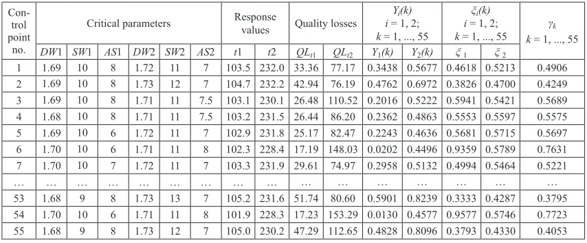
Table 1. A part of critical parameters and response values from a historical data, corresponding quality losses, principal component scores and data of grey relational analysis
Con-trol point
no.
Critical parameters Response values Quality losses i = 1, 2; Yi(k)
k = 1, ..., 55
ξi(k)
i = 1, 2;
k = 1, ..., 55 k = 1, ..., 55γk DW1 SW1 AS1 DW2 SW2 AS2 t1 t2 QLt1 QLt2 Y1(k) Y2(k) ξ 1 ξ 2
1 1.69 10 8 1.72 11 7 103.5 232.0 33.36 77.17 0.3438 0.5677 0.4618 0.5213 0.4906 2 1.69 10 8 1.73 12 7 104.7 232.2 42.94 76.19 0.4762 0.6972 0.3826 0.4700 0.4249 3 1.69 10 8 1.71 11 7.5 103.1 230.1 26.48 110.52 0.2016 0.5222 0.5941 0.5421 0.5689 4 1.68 10 8 1.71 11 7.5 103.2 231.5 26.44 86.20 0.2362 0.4863 0.5553 0.5597 0.5575 5 1.69 10 6 1.72 11 7 102.9 231.8 25.17 82.47 0.2243 0.4636 0.5681 0.5715 0.5697 6 1.70 10 6 1.71 11 8 102.3 228.4 17.19 148.03 0.0202 0.4496 0.9359 0.5789 0.7631 7 1.70 10 7 1.72 11 7 103.3 231.9 29.61 74.97 0.2958 0.5132 0.4994 0.5464 0.5221
… … … …
Coefficient ξi(k) was calculated by (5) and the Grey Relational Grade γk by using (6), where the weights (proportions) ωi are listed in Table 2. The
results of GRA are listed in Table 1.
Table 2. Results of PCA
Principal components PC1 PC2
Eigenvalues 1.0319 0.9681
Proportions 0.516 0.484
Eigenvectors NQL t1 0.707 0.707
NQL t2 -0.707 0.707
From γk and the factor values in Table 1, the factor effects can be tabulated. The optimal setting of each factor is the one that yields the highest multi-response performance measure, hence the optimal conditions obtained from the factor effects method was: DW1 = 1.70; SW1 = 11; AS1 = 6; DW2 = 1.71; SW2 = 11; AS2 = 8 [16].
Since the factor effects method discusses only discrete parameter values used in a historical data set, the above parameters setting was adopted as a basis to form the initial population in GA, to find the optimal solution in continual multi-dimensional space.
2.3 Implementation of the ANN&GA-Based Method
The set of BP ANNs were trained to model the relationship between synthetic performance measure γ and critical parameters. Each of the developed networks has six neurons in the input layer corresponding to six parameters, and one neuron in the output layer corresponding to a single synthetic multi-response performance measure. The number of neurons in the hidden layer varies from 1 to 9. The results of training of ANNs are presented in Table 3. The network with topology 6-5-1 showed the least error (MSE = 0.000588) and therefore it was selected to present the process model (Fig. 1) [16].
Fig.1. Topology of the selected ANN model
The selected network present an objective functions for GA. Nine GAs were developed; the initial population was seeded close to the set suggested by the factor effects method; population size was 30. The results of a tested GAs are given in Table 4. All the tested GAs showed the same result in terms of the best fitness value (γ = 0.88120) and the optimal parameters setting: DW1 = 1.70; SW1 = 11; AS1 = 5; DW2 = 1.71; SW2 = 11; AS2 = 9. This set is adopted as a final solution of the observed problem [16].
The results of different GAs show robustness with respect to GA’s own settings. Regarding the additional criteria, it could be seen that algorithms GA3, GA6 and GA9 that use ‘tournament‘ selection showed the lowest off-line performance. Since it was proven in previous studies that the loss of diversity increases with the increase of tournament size, and, from the other side, favourable selection intensity also increases with the increase of tournament size, in the observed study, it was decided to use the tournament size of 4. Almost identical results were obtained with the tournament size 2; however, tournament size 8 showed significantly lower off-line performance. One of the characteristics of a ‘tournament‘ selection is high variance in the distribution; ‘stochastic uniform‘ and ‘roulette‘ selection minimises this mean variance. These observations might be related to low off-line performance of GAs that use ‘tournament‘ selection in this study. However, interpretation of these results may be difficult as it depends on the optimisation problem.
Initial population in GA was formed in the proximity of the set suggested by the factor effects method. All GAs converged to the optimal solution in the first generation, which is a consequence of a good-seeded initial population. If the initial population was not set properly, the GA would need more generations to find the actual optimal solution.
2.4 Discussion
to some experimentation analysis method, such as RSM. Table 5 provides a comparison of the synthetic multi-response performance measure γ
and optimal parameters setting obtained from two methods of the analysis.
It could be seen that regarding the synthetic performance measure the intelligent method resulted in a better solution than the factor effects due to search over continual space within the specified bounds for parameters. The synthetic performance measure achieved by using optimal parameters setting obtained by the presented intelligent integrated approach (γ = 0.8211) is satisfactory, considering the fact that the maximum theoretical γ value is 1 (γk ∈ [ ; ]0 1 ) [16].
3 CONCLUSION
The paper presented two methods of the multi-response process optimisation for correlated responses, which employ historical data. Since the factor effects method could consider only
factor values used in a historical set, based on it the intelligent approach was developed to perform search in continual space of parameter solutions.
The major advantages of the presented factor effects method are [9], [16] and [19]:
• By using Taguchi’s SN ratio [20] and quality loss, relative significances of responses are adequately represented and the response mean and variation are assessed simultaneously.
• Multivariate statistical methods PCA and GRA are employed to uncorrelate and synthesise responses, ensuring that the weights of responses in synthetic performance measure are based on the total variance of the original data, which results in improved objectivity of the analysis.
In addition, the advantages of the ANN&GA-based method are [16] and [19]:
• The GA’s capacity of performing global search among all solutions in continual multi-dimensional space ensures convergence to the global optimal parameter settings.
Table 3. Results of training of ANNs (MSE and R values for ANNs with different topology)
Topology
of ANN 6-2-1 6-3-1 6-4-1 6-5-1 6-6-1 6-7-1 6-8-1 6-9-1
MSE 0.000882 0.0007232 0.000693 0.000588 0.000641 0.000715 0.000722 0.000732
R 0.9004 0.91028 0.93602 0.90797 0.91372 0.89458 0.91889 0.9104
Table 4. GAs settings and results
GA GA 1 GA 2 GA 3 GA 4 GA 5 GA 6 GA 7 GA 8 GA 9
Selection function Stochastic uniform Roulette wheel Tourna-ment Stochastic uniform Roulette wheel Tourna-ment Stochastic uniform Roulette wheel Tourna-ment Crossover function Single point Two point Arithmetic
Fitness function γ 0.82114 0.82114 0.82114 0.82114 0.82114 0.82114 0.82114 0.82114 0.82114 Off-line performance 0.82114 0.82114 0.55 0.82114 0.82114 0.56 0.82114 0.82114 0.59
Optimal
param-eters setting
DW1 1.7 1.7 1.7 1.7 1.7 1.7 1.7 1.7 1.7
SW1 11 11 11 11 11 11 11 11 11
AS1 5 5 5 5 5 5 5 5 5
DW2 1.71 1.71 1.71 1.71 1.71 1.71 1.71 1.71 1.71
SW2 11 11 11 11 11 11 11 11 11
AS2 9 9 9 9 9 9 9 9 9
Table 5. Comparative analysis of optimal parameter settings obtained by using two different methods
Method The factor effects method The ANN&GA-based method Optimal parameters setting [1.70; 11; 6; 1.71; 11; 8 ] [1.70; 11; 5; 1.71; 11; 9 ]
Synthetic multi-response
• The initial population in GA is formed in the proximity of the potentially good solution (the parameter settings obtained by the factor effects method), which advances the convergence to the global solution, meaning that the probability of finding the actual global parameters solution in the given number of generation is significantly improved. If the initial population was not defined at such way (e.g. if the initial population was randomly generated), in general, GA might not be able to find the actual global solution in a limited number of iterations.
• The proposed method does not depend on the type of the relations between responses and critical parameters, type and number of process parameters and responses, existence of correlations between responses or process parameters, or their interrelations.
The case study illustrated that the suggested approach can be effectively used to identify the optimal settings of critical parameters based on historical data, without any disruption caused by experimentation. The potential utility of the proposed integrated approach for process optimisation using historical data has increased because many companies today collect and store large quantities of a process data. On the other hand, the most significant limitation of the proposed approach is related to process data availability. In order to use this approach as an alterative to actual experimentation, it is necessary to monitor all parameters that are potentially critical for the observed responses and involve these data into corresponding control charts, prior to implementation of the proposed integrated approach.
4 REFERENCES
[1] Sukthomya, W., Tannock, J.D.T. (2005). Taguchi experimental design for manufacturing process optimization using historical data and neural network process model. International Journal of Quality &
Reliability Management, vol. 22, no. 5, p.
485-502.
[2] Guldi, R.L., Jenkins, C.D., Oamminga, G.M., Baum, T.A., Foster, T.A. (1989). Process optimization tweaking tool (POTT) and its
application in controlling oxidation thickness.
IEEE Transactions on Semiconductor
Manufacturing, vol. 2, no. 2, p. 54-59.
[3] Su, C.T., Tong, L.I. (1997). Multi-response robust design by principal component analysis. Total Quality Management and
Business Excellence, vol. 8, no. 6, p. 409-416.
[4] Fung, C.P., Kang, P.C. (2005). Multi-response optimization in friction properties of PBT composites using Taguchi method and principle component analysis. J Mater Proc
Technol, vol. 170, no. 3, p. 602-610.
[5] Wang, C.H., Tong, L.I. (2005). Optimization of dynamic multi-response problems using grey multiple attribute decision making.
Quality Engineering, vol. 17, no. 1, p. 1-9.
[6] Wu, F.C. (2004). Optimising robust design for correlated quality characteristics. Int J
Adv Manuf Technol, vol. 24, no. 1-2, p. 1-8.
[7] Hsieh, K.L. (2006). Parameter optimization of a multi-response process for lead frame manufacturing by employing artificial neural networks. Int J Adv Manuf Technol, vol. 28, p. 584-591.
[8] Hsu, C.M. (2001). Solving multi-response problems through neural networks and principal component analysis. Journal of the
Chinese Institute of Industrial Engineers, vol.
18, no. 5, p. 47-54.
[9] Sibalija, T., Majstorovic, V. (2009).
Multi-response optimisation of thermosonic copper wire-bonding process with correlated responses. Int J Adv Manuf Technol, vol. 42, no 3-4, p. 363-371.
[10] Roy, R., Mehnen, J. (2008). Dynamic multi-objective optimisation for machining gradient materials. Annals of the CIRP, vol. 57, no. 1, p. 429-432.
[11] Drain, D., Carlyle, W.M., Montgomery, D.C., Borror, C. Anderson-Cook, C. (2004). A genetic algorithm hybrid for constructing optimal response surface designs. Qual
Reliab Eng Int, vol. 20, no. 7, p. 637-650.
[12] Lau, H.C.W., Lee, C.K.M., Ip, W.H., Chan, F.T.S., Leung, R.W.K. (2005). Design and implementation of a process optimizer: a case study on monitoring molding operations.
Expert Systems, vol. 22, no. 1, p. 12-21.
mask manufacturing using NNPLS and genetic algorithm. Int J Prod Res, vol. 43, no. 15, p. 3209-3230.
[14] Hou, T.H., Chen, S.H., Lin, T.Y., Huang, K.M. (2006). An integrated system for setting the optimal parameters in IC chip-package wire bonding processes. Int J Adv Manuf
Technol, vol. 30, no. 3-4, p. 247-253.
[15] Tong, K.W., Kwong, C.K., Yu, K.M. (2004). Intelligent process design system for the transfer moulding of electronic packages. Int
J Prod Res, vol. 42, no. 10, p. 1911-1931.
[16] Šibalija, T. (2009). Development of an
intelligent designer of experiment model for application of Taguchi method. PhD thesis, Faculty of Mechanical Engineering, University of Belgrade (in Serbian).
[17] Taguchi, G. (1986). Introduction to quality engineering. Asian Productivity Organization, UNIPUB, New York.
[18] Ortiz, F., Simposon, J.R., Pigatiello, J.J., Heredia-Lagner, A. (2004). A genetic algorithm approach to multi-response optimisation. J Qual Technol, vol. 36, no. 4, p. 432-450.
[19] Sibalija, T., Majstorovic, V., Miljkovic, Z.
(2010). An intelligent approach to robust multiresponse process design. Int J Prod Res doi: 10.1080/00207543.2010.511476.
[20] Motorcu, A.R. (2010). The optimization of machining parameters using the taguchi method for surface roughness of AISI 8660 hardened alloy steel. Strojniški vestnik -
Journal of Mechanical Engineering, vol. 56,