The singular dynamic method for dynamic contact of thin elastic structures

A. Heibig, F. Filbet, L. I. Palade, Editors

THE SINGULAR DYNAMIC METHOD FOR DYNAMIC CONTACT OF

THIN ELASTIC STRUCTURES

C´

edric Pozzolini

_{, Yves Renard}

_{et Michel Sala¨}

_un

Abstract. This paper adresses the approximation of the dynamic impact of thin elastic structures. The principle of the presented method is the use of a singular mass matrix obtained by different discretizations of the deflection and velocity. The obtained semi-discretized problem is proved to be well-posed and energy conserving. The method is applied on some membrane, beam and plate models and associated numerical experiments are discussed.

Introduction

When the discretization of impact of elastic structures is addressed, it is generally noted that the vast majority of traditional time integration schemes show spurious oscillations on the contact displacement and stress (see for instance [7, 8, 11]). Moreover, these oscillations do not disappear when the time step decreases. Conversely, they tend to increase which is a characteristic of order two hyperbolic equations with unilateral constraints that makes it very difficult to build stable numerical schemes. These difficulties have already led to many researches under which a variety of solutions were proposed. Some of them consist in adding damping terms (see [27] for instance), but with a loss of accuracy on the solution, or to implicit the contact stress [4, 5] but with a loss of kinetic energy which could be independent of the discretization parameters (see the numerical experiments). Some energy conserving schemes have also been proposed in [7,8,10,15,16,28]. Unfortunately, these schemes, although more satisfactory than most of the other ones, lead to large oscillations on the contact stress. Besides, most of them do not strictly respect the constraint.

In this paper, we describe a class of methods whose principle is to make different approximations of the solution and of its time derivative. Such a principle was already studied for linear elastody-namics in [9]. Compared to the classical space semi-discretization, this corresponds to a singular modification of the mass matrix. In this sense, it is in the same class of methods than the mass redistribution method proposed in [11, 12] for elastodynamic contact problems. The main feature is to provide a well-posed space semi-discretization. The numerical tests show that it has a crucial influence on the stability of standard schemes and on the quality of the approximation, especially for the computation of Lagrange multipliers corresponding to the constraints.

The method is first described on an abstract hyperbolic equation on which the well-posedness of the semi-discretized problem by finite elements is proven. The method is then described on several models of thin elastic structures, namely membrane, Euler-Bernouilli beam and Kirchhoff-Love plate models. Some numerical tests for all these models are given and discussed. Finally, we present some perspectives and open problems.

1

Universit´e de Lyon, CNRS, INSA-Lyon, ICJ UMR5208, F-69621 Villeurbanne, France, [email protected]

2

Universit´e de Lyon, CNRS, INSA-Lyon, ICJ UMR5208, LaMCoS UMR5259, F-69621 Villeurbanne, France, [email protected]

3

Universit´e de Toulouse ; INSA, UPS, EMAC, ISAE ; ICA (Institut Cl´ement Ader), 10 Avenue Edouard Belin, F-31055 Toulouse, France,[email protected]

c

EDP Sciences, SMAI 2013

1.

_{The method for an abstract hyperbolic equation}

The method is introduced in [25] on the following abstract hyperbolic problem. Let Ω⊂Rd be a Lipschitz domain andH =L2_{(Ω) the standard Hilbert space of square integrable functions on Ω.}

LetW be a Hilbert space such that W ⊂H ⊂W′_{, with dense compact and continuous inclusions} and letA:W →W′ _{be a linear self-adjoint elliptic continuous operator. We consider the following} problem



   

   

Findu: [0, T]→K such that

∂2u

∂t2(t) +Au(t)∈f−NK(u(t)) , for a.e. t∈ (0, T] ,

u(0) =u0 ,

∂u

∂t(0) =v0 ,

(1)

whereK is a closed convex nonempty subset of W,f ∈W′

,u0∈K, v0∈H, T >0 andNK(u) is the normal cone toK defined by (see for instance [3] for more details)

NK(u) =

∅ , ifu /∈K , {f ∈W′_{:hf, w−ui}

W′_{, W} ≤0 , ∀w∈K} , ifu∈K .

This means that u(t) satisfies the second order hyperbolic equation and is constrained to remain in the convex K. There is no general result of existence nor uniqueness for the solution to this problem. Some existence results for a scalar Signorini problem can be found in [14, 17]. Introducing now the linear and bilinear symmetric maps

l(v) = hf, vi_W′_{, W} , a(u, v) = hAu, vi_W′_{, W} ,

Problem (1) can be rewritten as the following variational inequality:



   

   

Findu: [0, T]→K such that for a.e. t∈ (0, T]

h∂

2_u

∂t2(t), w−u(t)iW′_{, W}+a(u(t), w−u(t))≥l(w−u(t)) , ∀w∈K ,

u(0) =u0 ,

∂u

∂t(0) =v0 .

(2)

Note that the terminology “variational inequality” is used here in the sense that Problem (1) derives from the conservation of the energy functional

J(t) = 1 2

Z

Ω

(∂u

∂t(t))

2_dx+1

2a(u(t), u(t))−l(u(t)) +IK(u(t)) ,

whereIK(u(t)) is the convex indicator function ofK. However, it is generally not possible to prove that each solution to Problem (2) is energy conserving, due to the weak regularity involved.

2.

_{Approximation and well-posedness result}

The aim of this section is to present well-posed space semi-discretizations of Problem (2). The

adopted strategy is to use a Galerkin method with different approximations of u and ofv = ∂u

∂t.

LetWh_andHh_{be two finite dimensional vector subspaces ofW andH respectively. LetK}h_⊂Wh be a closed convex nonempty approximation ofK. The proposed approximation of Problem (2) is the following mixed approximation:



       

       

Finduh_{: [0, T]→K}h _andvh_{: [0, T]→H}h _{such that}

Z

Ω

∂vh ∂t (w

h_−uh_)dx+a(uh_{, w}h_−uh_)≥l(wh_−uh_{) , ∀w}h_∈Kh _{, ∀t∈ (0, T] ,}

Z

Ω

(vh−∂u

h

∂t )q

h_{dx= 0 , ∀q}h_∈Hh _{, ∀t∈ (0, T] ,}

uh_{(0) =u}h

0 , vh(0) =vh0 ,

whereuh0 ∈Kh andv0h ∈Hh are some approximations of u0 and v0 respectively. Of course, when

Hh_=Wh _{, this corresponds to a standard Galerkin approximation of Problem (2).}

Letϕi , 1≤i≤NW , andψi , 1≤i≤NH , be some basis ofWh andHh respectively, and let the matricesA, B andC, of sizesNW×NW ,NH×NW andNH×NH respectively, and the vectors L,U andV, of sizeNW ,NW andNH respectively, be defined by

Ai,j=a(ϕi, ϕj) , Bi,j=

Z

Ω

ψiϕjdx , Ci,j=

Z

Ω

ψiψjdx ,

Li=l(ϕi) , uh= NW

X

i=1

Uiϕi , vh= NH

X

i=1

Viψi .

Then, U and V are linked by the equation CV(t) = BU˙(t). So V can be eliminated since C is always invertible, which leads to the relationV(t) =C−1BU˙(t). Consequently, Problem (3) can be rewritten as



  

  

FindU : [0, T]→Khsuch that

(W −U(t))T(MU¨(t) +AU(t))≥(W −U(t))TL , ∀W ∈Kh , ∀t∈ (0, T] ,

U(0) =U0 , BU˙(0) =CV0 .

(4)

In comparison with the standard approximation whereHh_=Wh_{, the only difference introduced}

by the presented method is to replace the standard mass matrix

Z

Ω

ϕiϕjdx

i,j

byM =BTC−1B.

In the interesting cases where dim(Hh_)<dim(Wh_{), it corresponds to replace the standard invertible} mass matrix by a singular one.

Although the analysis could probably be extended to more complex situations, we assume that

Khis defined by a finite number of linear constraints as

Kh={wh∈Wh:gi(wh)≤αi , 1≤i≤Ng} ,

whereαi_∈Randgi_:Wh_{→R, 1≤i≤N}

g, are some linearly independent linear maps. Of course, this restricts the possibilities concerning the convexKsinceKh_{is supposed to be an approximation} ofK. With vector notations, this leads to

Kh={W ∈RNW _{: (G}i₎T_{W ≤α}

i , 1≤i≤Ng} ,

where Gi _{∈ R}NW _{are such that g}i_(wh_{) = (G}i₎T_{W, 1} ≤ _i ≤ _N

g . We will also denote by G the NW ×Ng matrix whose components are

Gij = (Gi)j .

Let us consider the subspaceFh _ofWh_{defined by}

Fh=

wh∈Wh:

Z

Ω

whqh= 0, ∀qh∈Hh

.

Then, the corresponding setF =

(

W ∈RNW _: NW

X

i=1

Wiϕi ∈Fh

)

is such that F = Ker(B). In this

framework, we consider the following condition:

inf Q∈RNg

Q6=0

sup W∈F W6=0

QTGW

||Q|| ||W|| > 0 , (5)

thatGis surjective onF. A direct consequence is that it implies dim(Fh)≥Ng and consequently

dim(Hh) ≤ dim(Wh) − Ng .

This again prescribes some conditions on the approximations which linkWh_,Hh_{and alsoK}h_{. We} will see in Section 3 that this condition can be satisfied for interesting practical situations. We can now prove the following result:

Theorem 1. If Wh_,Hh _andKh _{satisfy condition (5), then Problem (4) admits a unique solution.} Moreover, this solution is Lipschitz-continuous with respect tot.

Proof of this theorem can be found in [25]. In particular, it is based on the following result allowing a decomposition of the solution:

Lemma 1. IfWh_,Hh _andKh _{satisfy condition (5), then there exists a sub-space ofR}NW_{, sayF}c_,

such thatFc_{⊂Ker(G) and such thatF andF}c _{are complementary sub-spaces.}

Moreover, the following energy conservation is proved:

Theorem 2. If Wh_{, H}h _{and K}h _{satisfy condition (5), then the solution U(t) to Problem (4) is} energy conserving in the sense that the discrete energy

Jh(t) = 1 2U˙

T

(t)MU˙(t) +1 2U

T

(t)AU(t)−UT(t)L ,

is constant with respect tot.

3.

_{Application to a membrane model}

This section provides a simple but interesting situation for which some consistent approximations satisfy the condition (5). WhenW =H1_{(Ω) and K={w∈W :w≥0 a.e. on Ω}, we consider the}

following problem



          

          

Findu: [0, T]→K such that

∂2_u

∂t2(t)−∆u(t)∈f−NK(u(t)) in Ω , for a.e. t∈ (0, T] ,

∂u

∂n = 0 on ΓN ,

u= 0 on ΓD ,

u(0) =u0 ,

∂u

∂t(0) =v0 ,

where ΓN and ΓD is a partition of ∂Ω, ΓD being of non zero measure in ∂Ω. This models for instance the contact between an antiplane elastic structure with a rigid foundation or a stretched drum membrane under an obstacle condition. In this situation, the mass redistribution method presented in [12] is not usable since the area subjected to potential contact is the whole domain. Consequently, this method would lead to suppress the mass on the whole domain which is a non consistent drastic change of the problem.

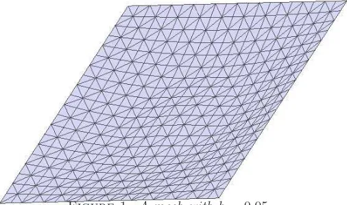
We build now the approximation spaces thanks to finite element method. Let Th _{a regular}

triangular mesh of Ω (in the sense of Ciarlet [2],hbeing the diameter of the largest element) and

Wh _{be the followingP}

1+ finite element space

Wh=







wh∈C0_{(Ω) :w}h₌ X

ai∈A

wiϕi+

X

T∈Th

wTϕT







,

whereA _{is the set of the vertices of the mesh which do not lie on Γ}

functions of aP1 Lagrange finite element method onTh. Each functionϕT, T ∈Th, is the cubic bubble function whose support isT. LetHh_{be the P}

0 finite element space

Hh=







vh∈L2_{(Ω) :v}h₌ X

T∈Th

vT1IT







,

and, finally, letKh _{be defined as}

Kh=

wh∈Wh:wh(ai)≥0 , for allai∈A , (6)

which means that the constraints are only prescribed at the vertices of the mesh. Then, it is proved in [25] that this choice ofWh_,Hh _andKh_{satisfies condition (5).}

4.

_{Extension to the vibro-impact of structures on rigid obstacles}

4.1.

Case of a beam

In [23], the method is applied to the fourth order problem of the dynamical evolution of an Euler-Bernouilli beam evolving between two rigid obstacles. The considered unknown is the vertical deflection, which is constrained to belong to

K={w∈H2_{(0, L) :g}

1(x)≤w(x)≤g2(x) , for allx∈[0, L]} ,

whereg1 andg2 are two maps from [0, L] to ¯R:=R∪ {−∞,+∞}such that

g1(x) < 0 < g2(x) , ∀x∈[0, L] .

These maps denote the position of the obstacles. If u(x, t) is the vertical deflection, the strong formulation of the problem, in the case of a clamped-free beam, reads as

                    

Findu: [0, T]→K such that

ρS ∂

2_u

∂t2(t) + EI

∂4_u

∂x4(x, t) ∈ f−NK(u(t)) , ∀(x, t)∈[0, L]×(0, T] ,

u(x,0) =u0(x) ,

∂u

∂t(x,0) =v0(x) , ∀x∈[0, L] ,

u(0, t) =∂u

∂x(0, t) = ∂2u

∂x2(L, t) =

∂3u

∂x3(L, t) = 0 , ∀t∈(0, T] ,

where ρ >0 is the mass density, E is the Young modulus, while S and I are the surface and the inertial momentum of the beam section, respectively.

The weak form of this problem can be written as

                  

Findu: [0, T]→K0 andv: [0, T]→L2(0, L) such that for a.e. t∈(0, T]

Z L

0 h

ρS ∂v

∂t (w−u) + EI ∂2_u

∂x2

∂2_(w−u)

∂x2 i

dx ≥

Z L

0

f (w−u)dx , ∀w∈K0 ,

Z L

0

(v−∂u

∂t)q dx = 0 , ∀q∈L

2_{(0, L) ,}

u(x,0) =u0(x)∈K0 , v(x,0) =v0(x)∈L2(0, L) , ∀x∈[0, L] ,

whereK0={w∈K:w(0) =w′(0) = 0}.

To build the finite element method, it is introduced a partition of [0, L] into N subintervals of lengthh = L/N, built on nodes xi = ih, for 0 ≤ i ≤ N. As nodex0 = 0 is clamped, we

will omit it from now on and consider that indexi varies between 1 and N. Otherwise, it would introduce small modifications in the following. So, at each node xi are associated two Hermite piecewise cubic functions, sayφ2i−1 andφ2i , defined for 1 ≤ i ≤ N by

Moreover, functions φj are chosen of classC1 on [0, L], which insures that each φj belongs to the continuous spaceW ={H2_{(0, L) :w(0) =w}′_{(0) = 0}. Hence, displacementw}h _reads

wh(x) = N

X

i=1

wh2i−1φ2i−1(x) +

N

X

i=1

w2hiφ2i(x) ,

and coefficientwh

2i−1 gives the value ofwh at nodexi whilewh2i gives the value of its derivative at the same node. The approximation space for displacements is then

Wh = span{φj , 1≤j≤2N} .

Let us now explain how the approximation Kh _{of K}

0 is obtained. Following the idea of the

previous section, unilateral constraints are only considered at the nodes of the mesh. It means convexKh _is

Kh = {wh∈Wh/ g1(xi) ≤ wh(xi) ≤ g2(xi) , ∀i∈[0, N]} .

With vector notations, settingα−

i ≡ g1(xi) andαi+ ≡ g2(xi) for alli, this space may be written (we keep the same notation for simplicity)

Kh = {W ∈RNW _{/ α}−

i ≤ (Gi)T W ≤α

+

i , ∀i∈[0, N]} ,

whereGi _{is the vector ofR}NW _{such that (G}i₎T _{W = w}h_(x

i), for all nodexi .

It is proved in [23] that such a nodal contact condition together with the use of the cubic Hermite element for the deflection and either a piecewise constant finite element method, or a continuous linear one, for the velocity satisfy the inf-sup condition (5).

Remark 1. Since we deal with a fourth order problem with respect to the space derivative, it is not possible to consider a linear space approximation. In fact, for this beam model, we use the classical Hermite third degree polynomials to approximate the numerical displacement. In the above approximation ofK, as we consider only constraints on node displacements, the effect of the derivatives, namely the curvature, is not taken into account. Then, in this framework, the beam could cross the obstacle between two nodes, but we shall neglect this aspect in the following.

4.2.

Case of a plate

Let us consider a thin elastic plate. For this kind of structures, starting froma priorihypotheses on the expression of the displacement fields, a two-dimensional problem is usually derived from the three-dimensional elasticity formulation by means of integration along the thickness, say 2ε. For the Kirchhoff-Love plate model, the only variable is the normal deflection, say u(x, t), and is set down on the mid-plane of the plate Ω. So the Kirchhoff-Love elastodynamical model reads as



  

  

Findu = u(x, t) with (x, t) ∈ Ω × (0, T] such that for anyw∈W

Z

Ω

2ρε ∂

2_u

∂t2 w dx + a(u, w) = Z

Ω

f w dx ,

where

a(u, w) =

Z

Ω

2 E ε3

3 (1−ν2₎

(1−ν) ∂

2_u

∂xα∂xβ

+ ν ∆u δαβ

∂2_w

∂xα ∂xβ dx ,

where the mechanical constants, for a plate made of a homogeneous and isotropic material, are its Young modulusE, its Poisson ratioνand its mass densityρ. Moreover,δαβis the Kronecker symbol and the summation convention over repeated indices is adopted, Greek indices varying in{1,2}. If the plate is assumed to be clamped on a non-zero measure part of the boundary∂Ω denoted Γc and free on Γf , such as∂Ω = Γc ∪ Γf , the space of admissible displacements is

W = { w∈H2_{(Ω) / w(x) = 0 = ∂}

where∂nwis the normal derivative along Γc . Finally, the associated initial conditions are

u(x,0) = u0(x) ,

∂u

∂t(x,0) = v0(x) , ∀x ∈ Ω .

Let us now introduce the dynamic frictionless Kirchhoff-Love equation with Signorini contact conditions along the plate. We assume that the plate motion is also limited by rigid obstacles located above and below the plate. So, the displacement is constrained to belong to the convex set

K = {w∈W : g1(x) ≤ w(x) ≤ g2(x) , ∀x∈Ω} ,

where g1 and g2 are two maps which still satisfy g1(x) < 0 < g2(x), for all x ∈ Ω. Then, the

mechanical frictionless elastodynamic problem for a plate between two rigid obstacles can be written as the following variational inequality



         

         

Findu: [0, T]→K andv: [0, T]→L2_{(Ω) such for a.e. t∈(0, T]}

Z

Ω

2ρε ∂v

∂t (w−u)dx + a(u, w−u) ≥

Z

Ω

f (w−u)dx , ∀w∈K ,

Z

Ω

(v−∂u

∂t)q dx = 0 , ∀q∈L

2_{(Ω) ,}

u(x,0) = u0(x)∈K ,

∂u

∂t(x,0) = v0(x) , ∀x∈Ω .

Let us now introduce the space discretization of the displacement. As the Kirchhoff-Love model corresponds to a fourth order partial differential equation, a conformal finite element approximation needs the use of continuously differentiable elements. Among such ones (see [2]), the reduced HCT (Hsieh-Clough-Tocher) triangles and FVS (Fraeijs de Veubeke-Sanders) quadrangles are of particular interest. For the HCT (resp. FVS) element, the triangle (resp. quadrangle) is divided into three (resp. four) sub-triangles. The basis functions of these elements areP3 polynomials on each

sub-triangle and matchedC1_{across each internal edge. In addition, to decrease the number of degrees of}

freedom, the normal derivative is assumed to vary linearly along the external edges of the elements. Finally, both for triangles and quadrangles, there are only three degrees of freedom on each node: The value of the function and its first derivatives.

In [24], such elements for the deflection, piecewise constant velocity and still a nodal contact condition (as for beams) on each vertex of the mesh are numerically shown to satisfy the inf-sup condition (5).

5.

_{Numerical discussion}

5.1.

Midpoint schemes

As far as numerical results are concerned, in this paper, we mainly use a midpoint scheme for the time discretization of the problem. It is an interesting scheme since it is energy conserving on the linear part (equation without constraint) but, of course, any other stable scheme can be applied. For exemple, in [23] and [24], Newmark schemes are also used. So, if ∆t stands for the time step, the midpoint scheme, applied on all the previous problems, consists in findingUn+1/2 _inKh _such that



     

     

(W−Un+1/2₎T _{(M Z}n+1/2_+AUn+1/2_{) ≥ (W−U}n+1/2₎T _Fn _{, ∀W ∈K}h _,

Un+1/2 ₌ Un+Un +1

2 , V

n+1/2 ₌ Vn+Vn +1

2 ,

BUn+1 _{= BU}n_{+ ∆tCV}n+1/2 _{, CV}n+1 _{= CV}n_{+ ∆tBZ}n+1/2 _,

(7)

velocity at timek∆t. As matrix C is invertible, we have

Vn+1 = 2Vn+1/2 − Vn = 2C−1

B U

n+1_−Un

∆t − V

n _{= 4C}−1

B U

n+1/2_−Un

∆t − V

n _.

Moreover,Zn+1/2 _{can be eliminated in the following way}

M Zn+1/2 = BT C−1

B Zn+1/2 = BT C−1 CVn+1−CVn

∆t = B

T Vn+1−Vn

∆t ,

or more explicitly

M Zn+1/2 _{= 4B}T _C−1_B U

n+1/2_−Un

∆t2 −2B T V

n

∆t =

4 ∆t2M U

n+1/2₋ 4

∆t2M U n₋ 2

∆tB T _Vn_S.

Then, a new formulation of (7) is



             

             

Un _andVn _{being given, findU}n+1/2_∈Kh _{such that}

(W −Un+1/2₎T ₍ 4

△t2M U

n+1/2_+AUn+1/2_{) ≥ (W −U}n+1/2₎T _F¯n _{, ∀W ∈K}h _,

where ¯Fn _{= F}n₊ 4 ∆t2M U

n₊ 2 ∆tB

T _Vn

Un+1 _{= 2U}n+1/2_−Un _{, V}n+1 _{= 2C}−1_B U

n+1_−Un

∆t − V

n _.

Let us note that this variational inequality has always a unique solution even ifM is singular.

5.2.

Case of the membrane model

We present now some numerical experiments on the membrane problem, with

Ω = (0,1) × (0,1) , ΓD=∂Ω , ΓN =∅ , f =−0.6 .

The initial condition is u(x,0) = 0.02, ∂u

∂t(x,0) = 0, for all x ∈ Ω, and we consider a

non-homogeneous Dirichlet conditionu(x, t) = 0.02, for allx∈∂Ω.

0 0.1 0.2 0.3 0.4 0.5 0.6 0

0.01 0.02 0.03 0.04 0.05

t

total energy

dt = 0.01 dt = 0.001

0 0.2 0.4 0.6

−0.01 0 0.01 0.02 0.03 0.04 0.05

t

center point displacement

dt = 0.01 dt = 0.001

0 0.1 0.2 0.3 0.4 0.5 0.6 −0.5

−0.4 −0.3 −0.2 −0.1 0

t

center point contact stress

dt = 0.01 dt = 0.001

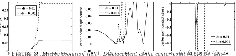
Figure 2. Energy evolution (left), Displacement at the center point(0.5,0.5) (cen-ter) and Contact stress at the center point (right) -P1+/P0method with a midpoint

scheme andh= 0.1.

The mesh, we used, is structured and can be viewed on Figure 1, where the solution is represented during the first impact on the obstacle. The numerical experiments are performed with our finite element library Getfem++ [26]. A semi-smooth Newton method is used to solve the discrete problem (see [1, 13]). All the numerical experiments use the same definition of convexKh_{, given by (6).}

The first numerical test is made with the midpoint scheme and the approximation presented in Section 3, that is aP1+/P0method (P1+ for displacement andP0 for velocity).

In good accordance with the theoretical results, the curves on Figure 2 show that the energy tends to be conserved when the time step decreases (an experiment with ∆t= 10−4 _{has been performed}

but the difference with the one for ∆t= 10−3 _{is not visible). Moreover, both the displacement and}

the contact stress, taken at the point (0.5,0.5), are smooth and converge satisfactorily when the time step decreases.

0 0.1 0.2 0.3 0.4 0.5 0.6 0

0.05 0.1 0.15 0.2 0.25

t

total energy

dt = 0.01 dt = 0.001

0 0.2 0.4 0.6

−0.01 0 0.01 0.02 0.03 0.04 0.05

t

center point displacement

dt = 0.01 dt = 0.001

0 0.1 0.2 0.3 0.4 0.5 0.6 −0.5

−0.4 −0.3 −0.2 −0.1 0

t

center point contact stress

dt = 0.01 dt = 0.001

Figure 3. Energy evolution (left), Displacement at the center point(0.5,0.5) (cen-ter) and Contact stress at the center point (right) -P1/P0 method with a midpoint

scheme andh= 0.1.

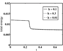
Conversely, the curves on Figure 3, obtained for a P1/P0 method, are unstable. The energy is

growing very fast after the first impact. The displacement and the contact stress are very oscillating and do not converge. Moreover, the instabilities are more important for the smallest time step. This method does not satisfy the condition (5) since dim(Hh_)≥dim(Wh_).

0 0.2 0.4 0.6 0

0.005 0.01 0.015 0.02

t

total energy

dt = 0.01 dt = 0.001 dt = 0.0001

0 0.2 0.4 0.6

−0.01 0 0.01 0.02 0.03 0.04 0.05

t

center point displacement

dt = 0.01 dt = 0.001 dt = 0.0001

0 0.1 0.2 0.3 0.4 0.5 0.6 −0.5

−0.4 −0.3 −0.2 −0.1 0

t

center point contact stress

dt = 0.01 dt = 0.001 dt = 0.0001

Figure 4. Energy evolution (left), Displacement at the center point(0.5,0.5) (cen-ter) and Contact stress at the center point (right) -P1+/P0method with a backward

Euler scheme andh= 0.1.

0 0.2 0.4 0.6

0 0.005 0.01 0.015 0.02

t

total energy

dt = 0.01 dt = 0.001 dt = 0.0001

0 0.2 0.4 0.6

−0.01 0 0.01 0.02 0.03 0.04 0.05

t

center point displacement

dt = 0.01 dt = 0.001 dt = 0.0001

0 0.1 0.2 0.3 0.4 0.5 0.6 −0.5

−0.4 −0.3 −0.2 −0.1 0

t

center point contact stress

dt = 0.01 dt = 0.001 dt = 0.0001

Figure 5. Energy evolution (left), Displacement at the center point(0.5,0.5) (cen-ter) and Contact stress at the center point (right) -P1/P0method with a backward

Euler scheme andh= 0.1.

0 0.2 0.4 0.6

0 0.005 0.01 0.015 0.02

t

total energy

h = 0.1 h = 0.3 h = 0.01

Figure 6. Energy evolution for a P1/P0 method, a backward Euler scheme and

∆t= 0.001, for different values of the mesh size.

5.3.

Case of a beam

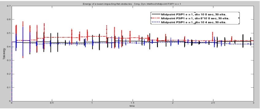
As in Dumont-Paoli [22], it is considered the case of a steel pipe, which length isL = 1.501 m, external diameter is equal to 1cmand thickness is 0.5mm. The material properties are characterized by its Young modulusE = 2.1011 _{P a and its density ρ = 8.10}3 _kg/m3_{. Thus, in this case, we}

have EI

ρS = 282.84m

4_.s−2_{, where I is the quadratic momentum of inertia of the beam and S its}

section. Moreover, in the following, we will consider flat obstacles all along the beam

g2(x) = −g1(x) = 0.1 , ∀x ∈ [0, L] .

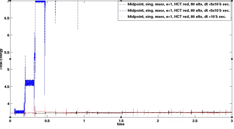
Figure 7. Energy for different time steps - P3/P0 singular mass matrix for Mid-point scheme. ∆t = 10−4 _,5.10−5 _,10−5 _{, 30/60/90 elements.}

Figure 8. Energy for different time steps - P3/P1 singular mass matrix for Mid-point scheme. ∆t = 10−4 _,5.10−5 _,10−5 _{, 30 elements.}

5.4.

Case of a plate

A steel rectangular panel is considered, of lengthL = 120cm, widthl = 40cmand thickness

ε = 0.5 cm. It means domain Ω is ]0, L[ × ]0, l[ . The flexural rigidity is D = 1.923 104_,

corresponding toE = 210 GP a andν = 0.3, while ρ = 7.77 103_kg/m3_{. This plate is clamped}

along one edge and free along the three others. Moreover, only the following kind of obstacle will be considered here. It is a flat obstacle under the whole plate, which reads

Finally, as we are mainly interested to study conservation of energy, we consider the case where there is no loadingf(x, t) ≡ 0 for all xand t. All energy is contained in an initial displacement

u0 , obtained as the static equilibrium of the plate under a constant loadf0 = 14600N and an

initial velocityv0 = 0.

In the following figures are given the energy evolutions for different time steps, for midpoint scheme with singular mass matrix. We notice that energy is weakly increasing and can be stabilized when the time step decreases. And the numericaly observed stability condition seems to be more restrictive for triangles than for quadrilaterals.

Figure 10. Energy for different time steps. Reduced FVS , 40 quadrilaterals. Midpoint scheme.

6.

_{Open problems and perspectives}

The semi-discretization, proposed here, leads to a problem which is equivalent to a regular Lip-schitz ordinary differential equation (see also [29] for a slightly different approach). This method generalizes in a sense the ones presented in [6, 12] with the advantage that no artificial modification of the mass matrix is necessary.

This is compared to the classical semi-discretizations, for example with finite element methods, which give a problem in time which is a measure differential inclusion (see [18–21]). Such a differential inclusion is systematically ill-posed, unless an additional impact law is considered.

Concerning thin structures, as it is illustrated by Figures 4, 5 and 6, numerical schemes do not necessarily converge toward the same solution. The limit solution may have different characteristics of impact energy loss. This suggests that in the case of thin structures, modeling of the restitution of the impact energy should be added to the impact law. The proposed semi-discretization being conservative in energy, it corresponds to a total restitution of the impact energy. A classical semi-discretization by finite elements with an implicit Euler scheme, as in Figure 6 corresponds to a certain loss of impact energy. Note that this energy loss is not necessarily maximal. Finally, the dissipation of the impact will certainly depend at the same time on the type of semi-discretization in space, the type of time integration scheme, the ratio between the space step and the time step, the kind of discretization of the contact conditions and finally of how the structure impacts the thin rigid obstacle (more or less obliquely, for instance). For the moment, the accurate modeling of the energy restitution at impact for the approximation of the dynamics of thin structures seems a little studied area. An interesting perspective is to try to characterize the different numerical schemes according to their characteristic in term of energy restitution.

References

[1] P. Alart, A. Curnier. A mixed formulation for frictional contact problems prone to Newton like solution methods.Comp. Meth. Appl. Mech. Engng., 92, pp. 353–375, 1991.

[2] P.G. Ciarlet.The finite element method for elliptic problems. Studies in Mathematics and its Applications No 4, North Holland, 1978.

[3] K. Deimling.Multivalued Differential Equations. de Gruyter, 1992.

[5] N.J. Carpenter.Lagrange constraints for transient finite element surface contact. Int. J. Num. Meth. Eng, 32, pp. 103–128, 1991.

[6] C. Hager, B. Wohlmuth.Analysis of a modified mass lumping method for the stabilization of frictional contact problems. to appear in SIAM J. Numer. Anal.

[7] P. Hauret.Numerical methods for the dynamic analysis of two-scale incompressible nonlinear structures. Th`ese de Doctorat, Ecole Polythechnique, France, 2004.

[8] P. Hauret, P. Le Tallec.Energy controlling time integration methods for nonlinear elastodynamics and low-velocity impact. Comput. Meth. Appl. Mech. Engrg., 195, pp. 4890–4916, 2006.

[9] T.J.R. Hugues, H. M. Hiler and R. L. Taylor.A reduction scheme for problems of structural dynamics. 12, pp. 749–767, 1976.

[10] T.J.R. Hugues, R. L. Taylor, J. L. Sackman, A. Curnier, W. Kanok-Nukulchai.A finite element method for a class of contact-impact problems. 8, pp. 249–276, 1976.

[11] H.B. Khenous. Probl`emes de contact unilat´eral avec frottement de Coulomb en ´elastostatique et ´elastodynamique. Etude math´ematique et r´esolution num´erique. PhD thesis, INSA de Toulouse, France, 2005. [12] H.B. Khenous, P. Laborde, Y. Renard.Mass redistribution method for finite element contact problems in

elastodynamics. Eur. J. Mech., A/Solids, 27(5), pp. 918–932, 2008.

[13] H.B. Khenous, J. Pommier, Y. Renard.Hybrid discretization of the Signorini problem with Coulomb friction. Theoretical aspects and comparison of some numerical solvers. Applied Numerical Mathematics, 56(2), pp. 163– 192, 2006.

[14] J.U. Kim.A boundary thin obstacle problem for a wave equation. Com. part. diff. eqs., 14(8&9), pp. 1011–1026, 1989.

[15] T.A. Laursen, V. Chawla.Design of energy conserving algorithms for frictionless dynamic contact problems. Int. J. Num. Meth. Engrg, 40, pp. 863–886, 1997.

[16] T.A. Laursen, G.R. Love.Improved implicit integrators for transient impact problems-geometric admissibility within the conserving framework. Int. J. Num. Meth. Eng., 53, pp. 245–274, 2002.

[17] G. Lebeau, M. Schatzman.A wave problem in a half-space with a unilateral constraint at the boundary. J. diff. eqs., 55, pp. 309–361, 1984.

[18] J.J. Moreau.Liaisons unilat´erales sans frottement et chocs in´elastiques. C.R.A.S. s´erie II, 296, pp. 1473–1476, 1983.

[19] J.J. Moreau.Numerical aspects of the sweeping process. Comp. Meth. Appl. Mech. Engrg., 177, pp. 329–349, 1999.

[20] L. Paoli.Time discretization of vibro-impact. Phil. Trans. R. Soc. Lond. A., 359, pp. 2405–2428, 2001. [21] L. Paoli, M. Schatzman.Approximation et existence en vibro-impact. C. R. Acad. Sci. Paris, S´er. I, 329, pp.

1103–1107, 1999.

[22] Y. Dumont, L. Paoli.Vibrations of a beam between obstacles: convergence of a fully discretized approximation. M2AN, 40(4), pp. 705–734, 2006.

[23] C. Pozzolini, M. Salaun.Some Energy conservative schemes for vibro-impacts of a beam on rigid obstacles. ESAIM: M2AN, 45, pp. 1163–1192, 2011.

[24] C. Pozzolini, Y. Renard, M. Salaun.Asymptotic energy preserving schemes schemes for the vibro-impacts of a plates between rigid obstacles. Submitted.

[25] Y. Renard.The singular dynamic method for constrained second order hyperbolic equations. Application to dynamic contact problems. J. Comput. Appl. Math., 234(3), pp. 906–923, 2010.

[26] Y. Renard, J. Pommier. Getfem++. An Open Source generic C++ library for finite element methods. http://home.gna.org/getfem.

[27] K. Schweizerhof, J.O. Hallquist, D. Stillman.Efficiency Refinements of Contact Strategies and Algorithms in Explicit Finite Element Programming. In Computational Plasticity, eds. Owen, Onate, Hinton, Pineridge Press, pp. 457–482, 1992.

[28] R. L. Taylor, P. Papadopoulos.On a finite element method for dynamic contact-impact problems. Int. J. for Num. Meth. Eng., 36, pp. 2123–2140, 1993.