Two-Layer Feature Reduction for Sparse-Group Lasso via
Decomposition of Convex Sets
Jie Wang [email protected]
Department of Electronic Engineering and Information Science University of Science and Technology of China
Hefei, Anhui, China
Zhanqiu Zhang [email protected]
Department of Electronic Engineering and Information Science University of Science and Technology of China
Hefei, Anhui, China
Jieping Ye [email protected]
Department of Computational Medicine and Bioinformatics Department of Electrical Engineering and Computer Science University of Michigan
Ann Arbor, MI 48109-2218, USA
Editor:Zhihua Zhang
Abstract
Sparse-Group Lasso (SGL) has been shown to be a powerful regression technique for si-multaneously discovering group and within-group sparse patterns by using a combination of the`1and`2norms. However, in large-scale applications, the complexity of the
regular-izers entails great computational challenges. In this paper, we propose a novel two-layer featurereduction method (TLFre) for SGL via a decomposition of its dual feasible set. The two-layer reduction is able to quickly identify the inactive groups and the inactive features, respectively, which are guaranteed to be absent from the sparse representation and can be removed from the optimization. Existing feature reduction methods are only applicable to sparse models with one sparsity-inducing regularizer. To our best knowledge, TLFre isthe first one that is capable of dealing withmultiple sparsity-inducing regularizers. Moreover, TLFre has a very low computational cost and can be integrated with any existing solvers. We also develop a screening method—called DPC (decomposition ofconvex set)—for non-negative Lasso. Experiments on both synthetic and real data sets show that TLFre and DPC improve the efficiency of SGL and nonnegative Lasso by several orders of magnitude. Keywords: Sparse, Sparse Group Lasso, Screening, Fenchel’s Dual, Decomposition, Convex Sets, Composite Function Optimization
1. Introduction
Sparse-Group Lasso (SGL) (Friedman et al.; Simon et al., 2013) is a powerful regression technique in identifying important groups and features simultaneously. To yield sparsity at both group and individual feature levels, SGL combines the Lasso (Tibshirani, 1996) and group Lasso (Yuan and Lin, 2006) penalties. In recent years, SGL has found great success in a wide range of applications, including but not limited to machine learning
c
(Vidyasagar, 2014; Yogatama and Smith, 2014), signal processing (Sprechmann et al., 2011), bioinformatics (Peng et al., 2010) etc. Many research efforts have been devoted to developing efficient solvers for SGL (Friedman et al.; Simon et al., 2013; Liu and Ye, 2010; Vincent and Hansen, 2014). However, when the feature dimension is extremely high, the complexity of the SGL regularizers imposes great computational challenges. Therefore, there is an increasingly urgent need for nontraditional techniques to address the challenges posed by the massive volume of the data sources.
Recently, El Ghaoui et al. (2012) proposed a promising feature reduction method, called
SAFE screening, to screen out the so-called inactive features, which have zero coefficients in the solution, from the optimization. Thus, the size of the data matrix needed for the training phase can be significantly reduced, which may lead to substantial improvement in the efficiency of solving sparse models. Inspired by SAFE, various exact and heuristic feature screening methods have been proposed for many sparse models such as Lasso (Wang et al., 2013; Liu et al., 2014; Tibshirani et al., 2012; Xiang and Ramadge, 2012), group Lasso (Wang et al., 2013; Wang et al.; Tibshirani et al., 2012), etc. It is worthwhile to mention that the discarded features by exact feature screening methods such as SAFE (El Ghaoui et al., 2012), DOME (Xiang and Ramadge, 2012) and EDPP (Wang et al., 2013) are guaranteed to have zero coefficients in the solution. However, heuristic feature screening methods like strong rule (Tibshirani et al., 2012) may mistakenly discard features that have nonzero coefficients in the solution. Thus, to compute the exact solutions, the authors propose to check the KKT conditions after the screening pass of strong rules. More recently, the idea of exact feature screening has been extended to exact sample screening, which screens out the nonsupport vectors in SVM (Ogawa et al., 2013; Wang et al., 2014) and LAD (Wang et al., 2014). As a promising data reduction tool, exact feature/sample screening would be of great practical importance because they can effectively reduce the data size without sacrificing the optimality (Ogawa et al., 2014).
However, all of the existing feature/sample screening methods are only applicable for the sparse models with one sparsity-inducing regularizer. In this paper, we propose an exact two-layer feature screening method, called TLFre, for the SGL problem. The first and second layer of TLFre aim to quickly identify the inactive groups and the inactive features, respectively, which are guaranteed to have zero coefficients in the solution. To the best of our knowledge, TLFre is the first screening method which is capable of dealing with multiple sparsity-inducing regularizers.
cones. Then, we formulate the estimation of the upper bounds via nonconvex optimization problems. We show that these nonconvex problems admit closed form solutions.
The rest of this paper is organized as follows. In Section 2, we briefly review some basics of the SGL problem. We then derive the Fenchel’s dual of SGL with nice geometric properties under the elegant framework of Fenchel’s Duality in Section 3. In Section 4, we develop the TLFre screening rule for SGL. To demonstrate the flexibility of the proposed framework, we extend TLFre to the nonnegative Lasso problem in Section 5. Experiments in Section 6 on both synthetic and real data demonstrate that the speedup gained by the proposed screening rules in solving SGL and nonnegative Lasso can be orders of magnitude. Please see the appendix for detailed proofs that are not presented in the main text.
Notation: Let k · k1,k · k and k · k∞ be the`1,`2 and`∞ norms, respectively. Denote by Bn
1,Bn, and B∞n the unit `1, `2, and`∞ norm balls inRn (we omit the superscript if it
is clear from the context). For a set C, let intC be its interior. If C is closed and convex, we define the projection operator as
PC(w) := argminu∈Ckw−uk.
We denote the indicator function ofC by
IC(w) =
(
0, ifw∈ C,
∞, otherwise.
Let Γ0(Rn) be the class of proper closed convex functions on Rn. Forf ∈Γ0(Rn), let ∂f
be its subdifferential. The domain of f is the set domf :={w:f(w)<∞}. For w ∈ Rn, let [w]
i be its ith component. More generally, if G ⊂ {1,2, . . . , n} is an
index set, we denote the corresponding subvector of w by [w]G ∈ R|G|, where |G| denotes
the number of elements inG. Forγ ∈R, let
sgn(γ) =
(
sign(γ), ifγ 6= 0, 0, otherwise.
We define
SGN(w) =
(
s∈Rn: [s]i ∈
(
sign([w]i), if [w]i 6= 0;
[−1,1], if [w]i = 0.
)
We denote by γ+ = max(γ,0). Then, for γ ≥0, the shrinkage operator Sγ(w) : Rn → Rn
can be written as
[Sγ(w)]i = (|[w]i| −γ)+sgn([w]i), i= 1, . . . , n. (1)
2. Basics and Motivation
In this section, we briefly review some basics of SGL. Let y∈ RN be the response vector
and X ∈RN×p be the matrix of features. With the group information available, the SGL
problem (Friedman et al.) is
min
β∈Rp
1 2
y−XG
g=1Xgβg
2
+λ1
XG
g=1 √
whereng is the number of features in thegth group,Xg∈RN×ng denotes the predictors in
that group with the corresponding coefficient vectorβg, andλ1, λ2are positive regularization
parameters. Without loss of generality, letλ1 =αλandλ2=λwithα >0. Then, problem
(2) becomes:
min
β∈Rp
1 2
y−XG
g=1Xgβg
2
+λ
αXG
g=1 √
ngkβgk+kβk1
. (3)
By the Lagrangian multipliers method (Boyd and Vandenberghe, 2004) (see the appendix), we can derive the dual problem of SGL as follows.
sup
θ
1 2kyk
2−1
2
y
λ−θ
2
(4)
s.t. XTgθ∈ Dαg :=α√ngB+B∞, g= 1, . . . , G.
It is well-known that the dual feasible set of Lasso is the intersection of closed half spaces (thus a polytope); for group Lasso, the dual feasible set is the intersection of ellipsoids. Sur-prisingly, the geometric properties of these dual feasible sets play fundamentally important roles in most of the existing screening methods for sparse models with one sparsity-inducing regularizer (Wang et al., 2014; Liu et al., 2014; Wang et al., 2013; El Ghaoui et al., 2012).
When we incorporate multiple sparse-inducing regularizers to the sparse models, prob-lem (4) indicates that the dual feasible set can be much more complicated. Although (4) provides a geometric description of the dual feasible set of SGL, it is not suitable for fur-ther analysis. Notice that, even the feasibility of a given point θ is not easy to determine, since it is nontrivial to tell if XTgθ can be decomposed intob1+b2 with b1 ∈α
√
ngB and b2 ∈ B∞. Therefore, to develop screening methods for SGL, it is desirable to gain deeper understanding of the sum of simple convex sets.
In the next section, we analyze the dual feasible set of SGL in depth via the Fenchel’s Duality Theorem. We show that for each XT
gθ∈ Dαg, Fenchel’s duality naturally leads to
an explicit decompositionXT
gθ=b1+b2, with one belonging toα √
ngBand the other one
belonging toB∞. This lays the foundation of the proposed screening method for SGL.
3. The Fenchel’s Dual Problem of SGL
Algorithm 1 Guidelines for developing TLFre.
1: Given a pair of parameter values (λ, α), we estimate a region Θ that contains the dual optimumθ∗(λ, α) of (4).
2: We solve the following two optimization problems:
s∗g = sup
ξg
{kS1(ξg)k:ξg ∈Ξg ⊇XTgΘ}, where XTgΘ ={XgTθ:θ∈Θ}, (5)
t∗gk = sup
θ
{|xTgkθ|:θ∈Θ}, where xgk is thek
th column of X
g. (6)
3: The TLFre screening rules take the form of
s∗g< α√ng⇒β∗g(λ, α) = 0, (7)
t∗gk ≤1⇒[βg∗(λ, α)]k= 0, (8)
whereβ∗(λ, α) is the optimal solution of SGL in (3).
3.1. The Fenchel’s Dual of SGL via Fenchel’s Duality Theorem
To derive the Fenchel’s dual problem of SGL, we need the Fenchel’s Duality Theorem as stated in Theorem 1. We denote the conjugate off ∈Γ0(Rn) by f∗ ∈Γ0(Rn):
f∗(z) = supwhw,zi −f(w). (9)
Theorem 1 [Fenchel’s Duality Theorem]Letf ∈Γ0(RN),Ω∈Γ0(Rp), andT(β) =y−Xβ
be an affine mapping fromRp toRN. Letp∗, d∗ ∈[−∞,∞]be primal and dual values defined,
respectively, by the Fenchel problems:
p∗ = infβ∈Rp f(y−Xβ) +λΩ(β); d∗ = supθ∈ RN −f
∗(λθ)−λΩ∗(XTθ) +λhy, θi.
One hasp∗≥d∗. If, furthermore, f andΩ satisfy the condition
0∈int (domf−y+Xdom Ω),
thenp∗=d∗, and the supreme is attained in the dual problem if finite.
We omit the proof of Theorem 1 as it is similar to that of Theorem 3.3.5 in (Borwein and Lewis, 2006).
Let f(w) = 12kwk2 andλΩ(β) be the second term in (3). We can write SGL as
minβ f(y−Xβ) +λΩ(β). (10)
Definition 2 (Bauschke and Combettes, 2011)Let h, g∈Γ0(Rn). The infimal convolution
of h andg is
(hg)(ξ) = infη h(η) +g(ξ−η), (11)
and it is exact at a point ξ if there exists a η∗(ξ) such that
(hg)(ξ) =h(η∗(ξ)) +g(ξ−η∗(ξ)). (12)
hg is exact if it is exact at each point in its domain, and we denote it by h g.
With the infimal convolution, we derive Ω∗ in the following Lemma.
Lemma 3 Let Ωα1(β) = αPG
g=1 √
ngkβgk, Ω2(β) = kβk1 and Ω(β) = Ωα1(β) + Ω2(β). Moreover, let Cα
g =α √
ngB ⊂Rng, g= 1, . . . , G. Then, the following hold:
(i) (Ωα1)∗(ξ) =PG
g=1ICgα(ξg), (Ω2)
∗(ξ) =PG
g=1IB∞(ξg),
(ii) Ω∗(ξ) = ((Ωα1)∗ (Ω2)∗) (ξ) =PGg=1 IB
ξ
g−PB∞(ξg)
α√ng
,
where ξg ∈Rng is the sub-vector of ξ corresponding to the gth group.
To prove Lemma 3, we first cite the following technical result.
Theorem 4 (Hiriart-Urruty, 2006) Let f1,· · · , fk ∈ Γ0(Rn). Suppose there is a point in
∩k
i=1domfi at whichf1,· · ·, fk−1 is continuous. Then, for all p∈Rn:
(f1+· · ·+fk)∗(p) = min p1+···+pk=p
[f1∗(p1) +· · ·+fk∗(pk)].
We now give the proof of Lemma 3.
Proof The first part can be derived directly by the definition as follows:
(Ωα1)∗(ξ) = sup
β
hβ, ξi −Ωα1(β) =
G
X
g=1
α√ng sup βg
βg,
ξg
α√ng
− kβgk
!
=
G
X
g=1
α√ngIB
ξg
α√ng
= G X g=1 IB ξg
α√ng
=
G
X
g=1 ICα
g(ξg).
(Ω2)∗(ξ) = sup β
hβ, ξi −Ω2(β) =IB∞(ξ) =
G
X
g=1
IB∞(ξg).
To show the second part, Theorem 4 indicates that we only need to show (Ωα1)∗(Ω2)∗(ξ)
is exact (note that Ωα1 and Ω2are continuous everywhere). Let us now compute (Ωα1)∗(Ω2)∗.
((Ωα1)∗(Ω2)∗) (ξ) =inf η (Ω
α
1)∗(ξ−η) + (Ω2)∗(η) (13)
= G X g=1 inf ηg IB
ξg−ηg
α√ng
+IB∞(ηg)
=
G
X
g=1
inf kηgk∞≤1
IB
ξg−ηg
α√ng
To solve the optimization problem in (13), i.e.,
µ∗g = inf
ηg
IB
ξg−ηg
α√ng
:kηgk∞≤1
, (14)
we can consider the following problem
νg∗= inf
ηg
1 α√ng
kξg−ηgk:kηgk∞≤1
. (15)
We can see that the optimal solution of problem (15) must also be an optimal solution of problem (14). Let η∗g(ξg) be the optimal solution of (15). We can see that η∗g(ξg) is indeed
the projection of ξg on B∞, which admits a closed form solution:
[ηg∗(ξg)]i= [PB∞(ξg)]i =
1, if [ξg]i>1,
[ξg]i, if|[ξg]i| ≤1, −1, if [ξg]i<−1.
Thus, problem (14) can be solved as
µ∗g =IB
ξg−PB∞(ξg)
α√ng
.
Hence, the infimal convolution in Eq. (13) is exact and Theorem 4 leads to
Ω∗(ξ) = ((Ωα1)∗ (Ω2)∗) (ξ) = G
X
g=1 IB
ξg−PB∞(ξg)
α√ng
, (16)
which completes the proof.
Note thatPB∞(ξg) admits a closed form solution:
[PB∞(ξg)]i = sgn ([ξg]i) min (|[ξg]i|,1).
By Theorem 1 and Lemma 3, we derive the Fenchel’s dual of SGL in Theorem 5 (see Section B for the proof).
Theorem 5 For the SGL problem in (3), the following hold:
(i) The Fenchel’s dual of SGL is given by:
inf
θ
1 2k
y
λ−θk
2−1
2kyk
2, (17)
s.t. XTgθ−PB∞(XTgθ)
≤α
√
ng, g= 1, . . . , G.
(ii) Let β∗(λ, α) and θ∗(λ, α) be the optimal solutions of problems (3) and (17), re-spectively. Then,
λθ∗(λ, α) =y−Xβ∗(λ, α), (18)
Eq. (18) and Eq. (19) are the so-called KKT conditions (Boyd and Vandenberghe, 2004) and can also be obtained by the Lagrangian multiplier method (see Section A in the ap-pendix).
Remark 6 We note that the shrinkage operator can also be expressed by
Sγ(w) =w−PγB∞(w), γ ≥0. (20)
Therefore, problem (17) can be written more compactly as
inf
θ
1 2k
y
λ−θk
2−1
2kyk
2, (21)
s.t. S1(XTgθ)
≤α
√
ng, g= 1, . . . , G.
The equivalence between the dual formulationsFor the SGL problem, its Lagrangian dual in (4) and Fenchel’s dual in (17) are indeed equivalent to each other. We bridge them together by the following lemma.
Lemma 7 (Bauschke and Combettes, 2011) Let C1 and C2 be nonempty subsets of Rn.
Then IC1 IC2 =IC1+C2.
In view of Lemmas 3 and 7, and recall thatDα
g =Cgα+B∞, we have
Ω∗(ξ) = ((Ωα1)∗ (Ω2)∗) (ξ) =
XG
g=1
ICα g IB∞
(ξg) =
XG
g=1 ID
α
g(ξg). (22)
Combining Eq. (22) and Theorem 1, we obtain the dual formulation of SGL in (4). There-fore, the dual formulations of SGL in (4) and (17) are the same.
Remark 8 An appealing advantage of the Fenchel’s dual in (17) is that we have a natural decomposition of all points ξg ∈ Dgα: ξg = PB∞(ξg) +S1(ξg)) with PB∞(ξg) ∈ B∞ and
S1(ξg)∈ Cgα. As a result, this leads to a convenient way to determine the feasibility of any dual variable θ by checking ifS1(XgTθ)∈ Cgα, g= 1, . . . , G.
3.2. Motivation of the Two-Layer Screening Rules
We motive the two-layer screening rules via the KKT condition in Eq. (19). As implied by the name, there are two layers in our method. The first layer aims to identify the inactive groups, and the second layer detects the inactive features for the remaining groups.
by Eq. (19), we have the following cases by noting ∂kwk1= SGN(w) and
∂kwk=
(n w
kwk
o
, ifw6= 0,
{u:kuk ≤1}, ifw= 0.
Case 1. Ifβ∗g(λ, α)6= 0, we have
[XTgθ∗(λ, α)]k∈
(
α√ng [β∗
g(λ,α)]k
kβ∗
g(λ,α)k + sign([β
∗
g(λ, α)]k), if [βg∗(λ, α)]k6= 0,
[−1,1], if [βg∗(λ, α)]k= 0.
In view of Eq. (23), we can see that
(a): S1(XTgθ∗(λ, α)) =α√ng
β∗g(λ1, λ2) kβ∗
g(λ1, λ2)k
andkS1(XTgθ∗(λ, α))k=α√ng, (24)
(b): If [XTgθ∗(λ, α]k
≤1 then [βg∗(λ, α)]k = 0. (25)
Case 2. Ifβ∗g(λ, α) = 0, we have
[XTgθ∗(λ, α)]k∈α √
ng[ug]k+ [−1,1],kugk ≤1. (26)
The first layer (group-level) of TLFre From (24) inCase 1, we have
S1(XTgθ∗(λ, α)) < α
√
ng ⇒βg∗(λ, α) = 0. (R1)
We can see that we can utilize (R1) to identify the inactive groups, and thus it is a group-level screening rule.
The second layer (feature-level) of TLFre Let xgk be the k
th column of X g. We
have [XTgθ∗(λ, α)]k=xTgkθ
∗(λ, α). In view of (25) and (26), we can see that
xTg
kθ
∗(λ, α)
≤1⇒[βg∗(λ, α)]k= 0. (R2)
Different from (R1), (R2) detects the inactive features, and thus it is a feature-level screening rule.
However, we cannot directly apply (R1) and (R2) to identify the inactive groups/features because both need to knowθ∗(λ, α). Inspired by the SAFE rules (El Ghaoui et al., 2012), we can first estimate a region Θ containing θ∗(λ, α). Let XTgΘ = {XTgθ : θ ∈ Θ}. Then, (R1) and (R2) can be relaxed as follows:
supξg
kS1(ξg)k:ξg ∈Ξg ⊇XTgΘ < α √
ng⇒β∗g(λ, α) = 0, (R1∗)
supθ
xTg
kθ
:θ∈Θ ≤1⇒[βg∗(λ, α)]k= 0. (R2∗)
We note that the two optimization problems in (R1∗) and (R2∗) are the same with (5) and (6), respectively. Therefore, inspired by (R1∗) and (R2∗), we can develop TLFre via the guidelines as shown in Algorithm 1.
3.3. The Effective Interval of Parameter Values
3.3.1. The Effective Interval of Parameter Values for Problem (3)
Consider the SGL problem in (3). For notational convenience, let
Fgα ={θ:kS1(XTgθ)k ≤α √
ng}, g= 1, . . . , G.
We denote the feasible set of the Fenchel’s dual of SGL by
Fα=∩g=1,...,GFgα.
Problem (17) [or (21)] implies that θ∗(λ, α) is the projection of y/λon Fα, i.e.,
θ∗(λ, α) =PFα(y/λ). (27)
Thus, if y/λ ∈ Fα, we have θ∗(λ, α) = y/λ. Moreover, (R1) implies that β∗(λ, α) = 0 if
y/λis an interior point ofFα. Indeed, we have the following stronger result.
Theorem 9 For the SGL problem in (3), let
λαmax= max
g {ρg :
S1(XTgy/ρg)
=α
√
ng}. (28)
Then, the following statements are equivalent:
(i) y λ ∈ F
α, (ii) θ∗(λ, α) = y
λ, (iii) β
∗(λ, α) = 0, (iv) λ≥λα max. Remark 10 Theorem 9 implies that the primal optimum β∗(λ, α) 6= 0 if and only if λ∈
(0, λαmax), namely, the effective interval of the parameterλwith a fixed value ofαis(0, λαmax).
We note that ρg in the definition ofλαmax admits a closed form solution. For notational
convenience, let |w| be the vector by taking absolute value of w component-wisely and [w](k) be the vector consisting of the first kcomponents of w.
Lemma 11 We sort 06=|XgTy| ∈Rng in descending order and denote it by z.
(i) If there exists [z]k such thatkS1(XTgy/[z]k)k=α √
ng, then ρg = [z]k.
(ii) Otherwise, letτi =kS1(XTgy/[z]i)k, i= 1, . . . , ng, andτng+1=∞. There exists a
k such that α√ng∈(τk, τk+1), andρg ∈([z]k+1,[z]k) is the root of
(k−α2ng)ρ2−2ρk[z](k)k1+k[z](k)k2 = 0.
We omit the proof of Lemma 11 because it is a direct consequence by noting that
kS1(XTgy/λ)k2 =α2ng
3.3.2. The Effective Interval of Parameter Values for Problem (2)
Theorem 9 implies that the optimal solution β∗(λ, α) is 0 as long as y/λ ∈ Fα. This
geometric property also leads to an explicit characterization of the set of (λ1, λ2) such that
the corresponding solution of problem (2) is 0. We denote by ¯β∗(λ1, λ2) the optimal solution
of problem (2).
Corollary 12 For the SGL problem in (2), let
λmax1 (λ2) = max g
1
√
ng
kSλ2(XTgy)k.
Then, the following hold.
(i) ¯β∗(λ1, λ2) = 0⇔λ1≥λmax1 (λ2).
(ii) ¯β∗(λ1, λ2) = 0 if
λ1 ≥λmax1 := maxg
1
√
ng
kXTgyk orλ2 ≥λmax2 :=kXTyk∞.
By Corollary 12, we can see that the primal optimum ¯β∗(λ1, λ2) 6= 0 if and only if
λ1 ∈ (0, λmax1 (λ2)). In other words, the effective interval of the parameter λ1 with a fixed
value of λ2 is (0, λmax1 (λ2)).
4. The Two-Layer Screening Rules for SGL
We follow the guidelines in Algorithm 1 to develop TLFre. In Section 4.1, we give an accurate estimation of θ∗(λ, α) via normal cones (Ruszczy´nski, 2006). Then, we compute the supreme values in (R1∗) and (R2∗) by solving nonconvex problems in Section 4.2.
We note that, in many applications, the parameter values that perform the best are usually unknown. To determine appropriate parameter values, commonly used approaches such as cross validation and stability selection involve solving SGL many times over a grip of parameter values. Thus, given {αi}Ii=1 and λi,1 >· · ·> λi,Ji, we can fix the value ofα
each time and solve SGL by varying the value of λ. We repeat the process until we solve SGL for all of the parameter values.
We present the TLFre screening rule combined with any solver for solving the SGL problems at a grid of parameters in Algorithm 2 (see Section 4.3 for a detailed explanation). Moreover, Theorem 9 gives the closed form solution ofβ∗(λ, α) for anyλ≥λαmax. Thus, we assume that the input parameter values in Algorithm 2 satisfyλi,j < λαmaxi for alli= 1, . . . ,I
Algorithm 2 The TLFre screening rule combined with any solver of SGL.
Input: {(λi,j, αi) : i = 1, . . . ,I, j = 1, . . . ,Ji}, where λαmaxi > λi,1 > · · · > λi,Ji for
i= 1, . . . ,I.
Output: β∗(λi,j, αi) and the index set Gi,j such that [β∗(λi,j, αi)]Gi,j = 0 for i= 1, . . . ,I
and j= 1, . . . ,Ji.
1: Initialize Gi,j ← ∅,i= 1, . . . ,I,j = 1, . . . ,Ji.
2: fori= 1 to I do
3: Compute λαi
max by Eq. (28) and setλi,0 ←λαmaxi .
4: Set θ∗(λi,0, αi)← λyi,0 by Theorem 9.
5: for j= 1 to Ji do
6: /* compute the ball Θ that containsθ∗(λi,j, αi) */
7: Compute v⊥αi(λi,j−1, λi,j) by Theorem 14.
8: Set the center of Θ: oαi(λi,j−1, λi,j)←θ
∗(λ
i,j−1, αi) + 12v⊥αi(λi,j, λi,j−1). 9: Set the radius of Θ: rαi(λi,j−1, λi,j)←
1 2kv
⊥
αi(λi,j, λi,j−1)k. 10: forg= 1 to Gdo
11: Compute s∗g(λi,j, λi,j−1;αi) by Theorem 17.
12: /* the first layer (group-level screening) of TLFre */
13: if s∗g(λi,j, λi,j−1;αi)< αi √
ng then
14: βg∗(λi,j, αi) = 0.
15: SetGi,j ← Gi,j∪ {gk:xgk is the k
th column of Xg}.
16: else
17: fork= 1 to ng do
18: Computet∗gk(λi,j, λi,j−1;αi) by Theorem 18.
19: /* the second layer (feature-level screening) of TLFre */
20: if t∗g
k(λi,j, λi,j−1;αi)≤1 then
21: [βg∗(λi,j, αi)]k= 0.
22: SetGi,j ← Gi,j∪ {gk}.
23: end if
24: end for
25: end if
26: end for
27: SetGi,j ← {k:k= 1, . . . , p, k /∈ Gi,j}.
28: Compute [β∗(λi,j, αi)]Gi,j on the reduced data set XGi,j by any solver. 29: Setθ∗(λi,j, αi)←(y−Xβ∗(λi,j, αi))/λi,j by Eq. (18).
30: end for
31: end for
4.1. Estimation of the Dual Optimal Solution
Due to the geometric property of the dual problem in (17), i.e., θ∗(λ, α) =PFα(y/λ), we
Proposition 13 (Ruszczy´nski, 2006; Bauschke and Combettes, 2011) For a closed convex set C ∈Rn and a point w∈ C, the normal cone to C at wis defined by
NC(w) ={v:hv,w0−wi ≤0,∀w0 ∈ C}. (29)
Then, the following hold:
(i) NC(w) ={v:PC(w+v) =w}.
(ii) PC(w+v) =w,∀v∈NC(w).
(iii) Let w∈ C/ . Then, w=PC(w)⇔w−w∈NC(w).
(iv) Let w∈ C/ andw=PC(w). Then, PC(w+t(w−w)) =w for all t≥0.
By Theorem 9, θ∗(¯λ, α) is known if ¯λ=λαmax. Thus, we can estimate θ∗(λ, α) in terms of θ∗(¯λ, α). Due to the same reason,we only consider the cases with λ < λαmax for θ∗(λ, α) to be estimated.
Theorem 14 For the SGL problem in (3), suppose that θ∗(¯λ, α) is known with λ¯≤λαmax. Let ρg, g= 1, . . . , G, be defined by Theorem 9. For λ∈(0,¯λ), let
nα(¯λ) =
y
¯ λ −θ
∗(¯λ, α), if ¯λ < λα max, X∗S1
XT∗ λαy
max
, if ¯λ=λαmax, whereX∗ = argmaxXgρg,
vα(λ,λ) =¯ y λ−θ
∗ (¯λ, α),
v⊥α(λ,λ) =¯ vα(λ,λ)¯ −hvα(λ,λ),¯ nα(¯λ)i knα(¯λ)k2
nα(¯λ).
Then, the following hold:
(i) nα(¯λ)∈NFα(θ∗(¯λ, α)),
(ii) kθ∗(λ, α)−(θ∗(¯λ, α) +12v⊥α(λ,λ))¯ k ≤ 12kvα⊥(λ,¯λ)k.
For notational convenience, we denote
oα(λ,λ) =¯ θ∗(¯λ, α) +
1 2v
⊥
α(λ,λ).¯ (30)
Theorem 14 shows that θ∗(λ, α) lies inside the ball of radius 12kv⊥α(λ,¯λ)k centered at
oα(λ,λ).¯
4.2. Solving for the Supreme Values via Nonconvex Optimization
We solve the optimization problems in (R1∗) and (R2∗). To simplify notations, let
Θ ={θ:kθ−oα(λ,λ)¯ k ≤
1 2kv
⊥
α(λ,λ)¯ k}, (31)
Ξg=
ξg :kξg−XTgoα(λ,λ)¯ k ≤
1 2kv
⊥
α(λ,λ)¯ kkXgk2
Theorem 14 indicates thatθ∗(λ, α)∈Θ. Moreover, we can see thatXTgΘ⊆Ξg,g= 1, . . . , G.
To develop the TLFre rule by (R1∗) and (R2∗), we need to solve the following optimization problems:
s∗g(λ,¯λ;α) = supξg{kS1(ξg)k:ξg ∈Ξg}, g= 1, . . . , G, (33)
t∗gk(λ,¯λ;α) =supθ{|xTgkθ|:θ∈Θ}, k= 1, . . . , ng, g= 1, . . . , G. (34)
4.2.1. The Solution of Problem (33)
We consider the following equivalent problem of (33):
1 2 s
∗
g(λ,λ;¯ α)
2
= supξg
1
2kS1(ξg)k
2 :ξ g ∈Ξg
. (35)
We can see that the objective function of problem (35) is continuously differentiable and the feasible set is a ball. Thus, problem (35) is nonconvex because we need tomaximize a convex function subject to a convex set. We first derive the necessary optimality conditions in Lemma 15 and then deduce the closed form solutions of problems (33) and (35) in Theorem 17.
Lemma 15 LetΞ∗g be the set of optimal solutions of (35) andξg∗ ∈Ξ∗g. Then, the following hold:
(i) Suppose that ξg∗ is an interior point of Ξg. Then, Ξg is a subset ofB∞.
(ii) Suppose thatξ∗g is a boundary point of Ξg. Then, there exists µ∗ ≥0 such that
S1(ξg∗) =µ∗ ξg∗−XTgoα(λ,λ)¯
. (36)
(iii) Suppose that there exists ξ0g ∈Ξg andξg0 ∈ B/ ∞. Then, we have
(iiia)ξg∗∈ B/ ∞ and ξg∗ is a boundary point of Ξg, i.e.,
kξg∗−XTgoα(λ,¯λ)k=
1 2kv
⊥
α(λ,¯λ)kkXgk2.
(iiib) The optimality condition in Eq. (36) holds with µ∗ >0.
To show Lemma 15, we need the following proposition.
Proposition 16 (Hiriart-Urruty, 1988) Suppose that h ∈ Γ0 and C is a nonempty closed convex set. If w∗ ∈ C is a local maximum ofh on C, then ∂h(w∗)⊆NC(w∗).
We now present the proof of Lemma 15.
Proof To simplify notations, let
c=XTgoα(λ,¯λ) andr=
1 2kv
⊥
α(λ,λ)¯ kkXgk2. (37)
By Eq. (1), we have
h(w) := 1
2kS1(w)k
2= 1
2
X
i
It is easy to see thath(·) is continuously differentiable. Indeed, we have
∇h(w) =S1(w). (39)
Then, problem (35) can be written as
1 2(s
∗
g(λ,¯λ;α))2= sup ξg
(
h(ξg) =
1 2
X
i
([ξg]i−1)2+: ξg ∈Ξg
)
, (40)
where Ξg ={ξg:kξg−ck ≤r}. Then, Proposition 16 results in
S1(ξg∗) =∇h(ξ∗g)⊆∂h(ξg∗)⊆NΞg(ξ
∗
g). (41)
(i) Suppose that ξg∗ is an interior point of Ξg. Then, we have NΞg(ξ
∗
g) = 0. By
Eq. (41), we can see that
0 =S1(ξg∗)⇒0 = 1 2kS1(ξ
∗
g)k2=
1 2(s
∗
g(λ,λ;¯ α))2 = sup ξg
1
2kS1(ξg)k
2:ξ g ∈Ξg
.
Therefore, we have
kS1(ξg)k= 0,∀ξg ∈Ξg. (42)
Because S1(ξg) =ξg−PB∞(ξg) (see Remark 6), Eq. (42) implies that
ξg =PB∞(ξg),∀ξg ∈Ξg ⇒ξg ∈ B∞,∀ξg ∈Ξg.
This completes the proof.
(ii) Suppose that ξg∗ is a boundary point of Ξg. We can see that
NΞg(ξ
∗
g) ={µ(ξg∗−c), µ≥0}. (43)
Then, Eq. (36) follows by combining Eq. (43) and the optimality condition in (41).
(iii) Suppose that there exists ξg0∈Ξg and ξg0 ∈ B/ ∞.
(iiia) The definition of ξg0 leads to
0<kS1(ξg0)k ≤ kS1(ξg∗)k ⇒ξg∗∈ B/ ∞.
Moreover, we can see that ξg∗ is a boundary point of Ξg. Because ifξ∗g is an
interior point of Ξg, the first part implies that Ξg ⊂ B∞. This contradicts with the existence of ξ0g. Thus, ξg∗ must be a boundary point of Ξg, i.e. kξg∗−ck=r.
(iiib) Because ξg∗ is a boundary point of Ξg, the second part implies that Eq. (36)
Based on the necessary optimality conditions in Lemma 15, we derive the closed form solutions of (33) and (35) in the following Theorem. The notations are the same as the ones in the proof of Lemma 15 [see Eq. (37) and Eq. (38)].
Theorem 17 For problems (33) and (35), letc=XTgoα(λ,¯λ),r= 12kv⊥α(λ,¯λ)kkXgk2 and
Ξ∗g be the set of the optimal solutions.
(i) Suppose that c∈ B/ ∞, i.e., kck∞>1. Let u=rS1(c)/kS1(c)k. Then,
s∗g(λ,¯λ;α) =kS1(c)k+r and Ξ∗g={c+u}. (44) (ii) Suppose that c is a boundary point of B∞, i.e., kck∞= 1. Then,
s∗g(λ,λ;¯ α) =r and Ξ∗g={c+u:u∈NB∞(c),kuk=r}. (45)
(iii) Suppose that c∈intB∞, i.e., kck∞<1. Let i∗∈ I∗={i:|[c]i|=kck∞}. Then,
s∗g(λ,λ;¯ α) = (kck∞+r−1)+, (46)
Ξ∗g=
Ξg, if Ξg⊂ B∞,
{c+r·sgn([c]i∗)ei∗ : i∗ ∈ I∗}, if Ξg6⊂ B∞andc6= 0,
{r·ei∗,−r·ei∗ : i∗ ∈ I∗}, if Ξg 6⊂ B∞andc= 0,
where ei is the ith standard basis vector.
Proof
(i) Suppose thatc∈ B/ ∞. By the third part of Lemma 15, we have
ξ∗g ∈ B/ ∞, kξ∗g−ck=r, (47)
ξ∗g−PB∞(ξ
∗
g) =S1(ξg∗) =µ
∗
(ξ∗g−c), µ∗ >0. (48)
By Eq. (48), we can see that µ∗ 6= 1 because otherwise we would have c =
PB∞(ξ
∗
g) ∈ B∞. Moreover, we can only consider the cases with µ∗ > 1 because kS1(ξ∗g)k = µ∗r and we aim to maximize kS1(ξ∗g)k. Therefore, if we can find a
solution withµ∗ >1, there is no need to consider the cases with µ∗∈(0,1).
Suppose that µ∗>1. Then, Eq. (48) leads to
c=PB∞(ξ
∗
g) +
1− 1
µ∗
ξg∗−PB∞(ξ
∗
g)
, (49)
ξg∗ =PB∞(ξ
∗
g) +
µ∗
µ∗−1 c−PB∞(ξ ∗
g)
. (50)
In view of part (iv) of Proposition 13 and Eq. (49), we have
PB∞(c) =PB∞(ξ
∗
Therefore, Eq. (50) can be rewritten as
S1(ξg∗) =ξg∗−PB∞(ξ
∗
g) =
µ∗
µ∗−1(c−PB∞(c)) =
µ∗
µ∗−1S1(c). (52) Combining Eq. (48) and Eq. (52), we have
µ∗
µ∗−1kS1(c)k=µ ∗k
ξ∗g−ck=µ∗r⇒µ∗ = 1 +kS1(c)k
r >1. (53)
The statement holds by plugging Eq. (53) and Eq. (51) into Eq. (50) and Eq. (52). Moreover, the above discussion implies that Ξ∗gonly contains one element as shown in Eq. (44).
(ii) Suppose that c is a boundary point of B∞. Then, we can find a point ξg0 ∈ Ξg
andξ0g ∈ B/ ∞. By the third part of Lemma 15, we also have Eq. (47) and Eq. (48) hold. We claim thatµ∗ ∈(0,1]. The argument is as follows.
Suppose that µ∗ >1. By the same argument as in the proof of the first part, we can see that Eq. (52) holds. BecauseS1(ξg∗)6= 0 by Eq. (47), we haveS1(c) 6= 0. This implies that c ∈ B/ ∞. Thus, we have a contradiction, which implies that µ∗ ∈(0,1].
Let us consider the cases with µ∗ = 1. Because kS1(ξg∗)k = µ∗r [see Eq. (48)] and we want to maximize kS1(ξg∗)k, there is no need to consider the cases with
µ∗ ∈ (0,1) if we can find solutions of problem (33) with µ∗ = 1. Therefore, Eq. (48) leads to
PB∞(ξ
∗
g) =c.
By part (iii) of Proposition 13, we can see that
PB∞(ξ
∗
g) =c⇔ξg∗−c∈NB∞(c). (54)
Combining Eq. (54) and Eq. (47), the statement holds immediately, which confirms thatµ∗ = 1.
(iii) Suppose that cis an interior point of B∞.
(a) We first consider the cases with Ξg ⊂ B∞. Then, we can see that
S1(ξ) = 0,∀ξ ∈Ξg ⇒Ξ∗g= Ξg.
In other words, an arbitrary point of Ξg is an optimal solution of problem
(33). Thus, we have
c+r·sgn(ei∗)ei∗ ∈Ξ∗g,
s∗g(λ,λ;¯ α) = 0.
On the other hand, we can see that
Therefore, we have
(kck∞+r−1)+= 0,
and thus
s∗g(λ,λ;¯ α) = (kck∞+r−1)+.
(b) Suppose that Ξg 6⊂ B∞, i.e., there exists ξ0 ∈Ξg such that ξ0 ∈ B/ ∞. By the third part of Lemma 15, we have Eq. (47) and Eq. (48) hold. Moreover, in view of the proof of the first and second part, we can see that µ∗ ∈ (0,1). Therefore, Eq. (48) leads to
(1−µ∗)ξg∗+µ∗c=PB∞(ξ
∗
g). (55)
By rearranging the terms of Eq. (55), we have
PB∞(ξ
∗
g)−c= (1−µ
∗
)(ξg∗−c). (56)
Because µ∗ ∈(0,1), Eq. (55) implies that PB∞(ξ
∗
g) lies on the line segment
connecting ξg∗ and c. Thus, we have
kξ∗g−PB∞(ξ
∗
g)k+kPB∞(ξ
∗
g)−ck=kξ
∗
g −ck=r. (57)
Therefore, to maximize kS1(ξg∗)k = kξg∗−PB∞(ξ
∗
g)k, we need to minimize kPB∞(ξ
∗
g)−ck. Because ξg∗ ∈ B/ ∞, we can see that PB∞(ξ
∗
g) is a boundary
point ofB∞. Therefore, we need to solve the following minimization problem:
min
φg
{kφg−ck:kφgk∞= 1}. (58)
Suppose thatc= 0. We can see that the set of optimal solutions of problem (58) is
Φ∗g ={ei}ng
i=1∪ {−ei} ng
i=1.
For each φ∗g ∈Φ∗g, we set it as PB∞(ξ
∗
g). In view of Eq. (56) and Eq. (47),
the statement follows immediately.
Suppose that c6= 0. Recall that I∗ ={i∗ :|[c]
i∗|=kck∞}. It is easy to see
that
Φ∗g =
(
φi∗: [φi∗]k= (
sgn([c]i∗), ifk=i∗,
[c]k, otherwise,
i∗ ∈ I∗
)
.
We can see that
φi∗−c= (1− |[c]i∗|)sgn([c]i∗)ei∗, i∗ ∈ I∗.
For each φi∗, we set it to PB
∞(ξ
∗
g). Then, we can see that the statement
4.2.2. The Solution of Problem (34)
Problem (34) can be solved directly via the Cauchy-Schwarz inequality.
Theorem 18 For problem (34), we have
t∗gk(λ,λ;¯ α) =|xTgkoα(λ,λ)¯ |+1 2kv
⊥
α(λ,λ)¯ kkxgkk.
We are now ready to present the proposed screening rule TLFre.
4.3. The Proposed Two-Layer Screening Rules
To develop the two-layer screening rules for SGL, we only need to plug the supreme values s∗g(λ,λ;¯ α) and tg∗k(λ,¯λ;α) in (R1∗) and (R2∗). We present the TLFre rule as follows.
Theorem 19 For the SGL problem in (3), suppose that we are given a grid of parameter values {αi}Ii=1 and λαmaxi = λi,0 > λi,1 > . . . > λi,Ji for each αi. Moreover, assume
that β∗(λi,j−1, αi) is known for an integer 0 < j < Ji. Let θ∗(λi,j−1, αi), vα⊥i(λi,j, λi,j−1)
and s∗g(λi,j, λi,j−1;αi) be given by Eq. (18), Theorems 14 and 17, respectively. Then, for
g= 1, . . . , G, the following holds
s∗g(λi,j, λi,j−1;αi)< αi √
ng ⇒βg∗(λi,j, αi) = 0. (L1) For the gth group that does not pass the rule in (L1), we have[βg∗(λi,j, αi)]k= 0 if
t∗gk(λi,j, λi,j−1;αi)≤1, (L2) where
t∗gk(λi,j, λi,j−1;αi)
=
xTgk
y−Xβ∗(λi,j−1, αi)
λi,j−1
+1 2v
⊥
αi(λi,j, λi,j−1)
+1 2kv
⊥
αi(λi,j, λi,j−1)kkxgkk.
(L1) and (L2) are the first and second layer screening rules of TLFre, respectively.
We also write Theorem 19 in an algorithmic manner in Algorithm 2. For each pair of parameter values (λi,j, αi), we first apply TLFre to identify the inactive groups and inactive
features, namely, the zero components of β∗(λi,j, αi). Then, we remove the inactive groups
and inactive features from the data matrix and apply an arbitrary solver to solve the SGL problem on the remaining features.
Specifically, lines 7 to 9 in Algorithm 2 compute the ball that contains θ∗(λi,j, αi) in
terms ofθ∗(λi,j−1, αi) (see remark 20). Lines 13 till 15 apply the first layer of TLFre, i.e., the
group-level screening, to identify the inactive groups. Take the gth group for an example. If the first layer identifies the gth group as an inactive group, we can set βg∗(λi,j, αi) = 0.
Otherwise, lines 20 till 23 apply the second layer of TLFre, i.e., the feature-level screening, to identify the inactive features in the gth group. The index set Gi,j stores the indices of inactive features, i.e., if k ∈ Gi,j, then [β∗(λi,j, αi)]k = 0. After we scan the entire
matrix, the index set Gi,j contains all the indices of inactive features identified by TLFre,
i.e., [β∗(λi,j, αi)]Gi,j = 0. Thus, the remaining unknowns are indeed [β
∗(λ
27). Then, we apply an arbitrary solver to solve for [β∗(λi,j, αi)]Gi,j on the reduced data
matrixXG
i,j, whereXGi,j = (xk1, . . . ,xkq),q =|Gi,j|, andk`∈ Gi,jfor`= 1, . . . , q. Once we
have solved for [β∗(λi,j, αi)]Gi,j, we indeed have solved forβ
∗(λ
i,j, αi) as [β∗(λi,j, αi)]Gi,j = 0.
Then, line 29 computesθ∗(λi,j, αi) by Eq. (18), based on which we can estimateθ∗(λi,j+1, αi)
and apply TLFre to identify the zero components ofβ∗(λi,j+1, αi).
Remark 20 As shown by Theorem 19 and Algorithm 2, TLFre estimates the dual optimum at (λi,j, αi), i.e., θ∗(λi,j, αi), in terms of a known dual optimum at a different pair of parameter values (λi,j−1, αi), i.e., θ∗(λi,j−1, αi). Then, we can apply TLFre to identify the inactive groups and inactive features and solve the TLFre problems on a reduced data matrix. Thus, to initialize TLFre, we may need to solve the SGL problem on the entire data matrix once to compute θ∗(λi,0, αi), which can be time consuming. However, we note that, Theorem 9 not only gives the effective interval of λ for a fixed value of α, but also a closed form solution of the dual optimum for any λ≥ λαmax. Thus, as we have done in Algorithm 2 (see line 3), we can always setλi,0 =λαmaxi andθ∗(λi,0, αi) =y/λi,0 to initialize the computation of TLFre. This implies that, if we combine TLFre and an arbitrary solver, we do not need to solve the SGL problem on the entire data matrix even once.
5. Extension to Nonnegative Lasso
The framework of TLFre is applicable to a large class of sparse models with multiple regu-larizers. As an example, we extend TLFre to nonnegative Lasso:
min
β∈Rp
1
2ky−Xβk
2+λkβk
1 : β ∈Rp+
, (59)
where λ >0 is the regularization parameter and Rp+ is the nonnegative orthant of Rp. In
Section 5.1, we transform the constraint β ∈ Rp+ to a regularizer and derive the Fenchel’s dual of the nonnegative Lasso problem. We then motivate the screening method—called DPC since the key step is todecompose a convex set via Fenchel’s Duality Theorem—via the KKT conditions in Section 5.2. In Section 5.3, we analyze the geometric properties of the dual problem and derive the set of parameter values leading to zero solutions. We then develop the screening method for nonnegative Lasso in Section 5.4.
5.1. The Fenchel’s Dual of Nonnegative Lasso
LetIRp
+ be the indicator function ofR p
+. By noting thatIRp+ =λIR
p
+ for anyλ >0, we can
rewrite the nonnegative Lasso problem in (59) as
min
β∈Rp
1
2ky−Xβk
2+λkβk
1+λIRp+(β). (60)
We now proceed by following a similar procedure as the one in Section 3.1. We note that the nonnegative Lasso problem in (60) can also be formulated as the one in (10) with f(·) = 12k · k2and Ω(β) =kβk
1+IRp+(β). To derive the Fenchel’s dual of nonnegative Lasso,
we need to findf∗ and Ω∗ by Theorem 1. Since we have already seen that f∗(·) = 12k · k2
in Section 3.1, we only need to find Ω∗(·). The following result is indeed a counterpart of Lemma 3.
Lemma 21 Let Ω2(β) =kβk1, Ω3=IRp
+(β), and Ω(β) = Ω2(β) + Ω3(β). Then,
(i) (Ω2)∗(ξ) =IB∞(ξ) and (Ω3)
∗(ξ) =I
Rp−(ξ), whereR
p
− is the nonpositive orthant of
Rp.
(ii) Ω∗(ξ) = ((Ω2)∗ (Ω3)∗)(ξ) =IRp
−(ξ−1), where R
p 31= (1,1, . . . ,1)T.
We omit the proof of Lemma 21 since it is very similar to that of Lemma 3.
Remark 22 Consider the second part of Lemma 21. Let C1 ={ξ :ξ ≤ 1}, where “≤” is defined component-wisely. We can see that
IRp
−(ξ−1) =IC1(ξ).
On the other hand, Lemma 7 implies that
Ω∗(ξ) = ((Ω2)∗ (Ω3)∗)(ξ) =IB∞+Rp−(ξ).
Thus, we haveB∞+Rp−=C1. The second part of Lemma 21 decomposes each ξ∈ B∞+Rp−
into two components: 1 andξ−1 that belong toB∞ and Rp−, respectively.
By Theorem 1 and Lemma 21, we can derive the Fenchel’s dual of nonnegative Lasso in the following theorem (which is indeed the counterpart of Theorem 5).
Theorem 23 For the nonnegative Lasso problem, the following hold:
(i) The Fenchel’s dual of nonnegative Lasso is given by:
inf
θ
1 2
y
λ−θ
2 −1
2kyk
2 :hx
i, θi ≤1, i= 1, . . . , p
. (61)
(ii) Let β∗(λ) and θ∗(λ) be the optimal solutions of problems (60) and (61), respec-tively.Then,
λθ∗(λ) =y−Xβ∗(λ), (62)
XTθ∗(λ)∈∂kβ∗(λ)k1+∂IRp
+(β
∗(λ)). (63)
5.2. Motivation of the Screening Method via KKT Conditions
The key to develop the DPC rule for nonnegative lasso is the KKT condition in (63). We can see that ∂kwk1= SGN(w) and
∂IRp
+(w) =
(
ξ ∈Rp : [ξ] i=
(
0, if [w]i >0,
ρ, ρ≤0, if [w]i = 0,
)
.
Therefore, the KKT condition in (63) implies that
hxi, θ∗(λ)i ∈
(
1, if [β∗(λ)]i >0,
%, %≤1, if [β∗(λ)]i = 0.
(64)
By Eq. (64), we have the following rule:
hxi, θ∗(λ)i<1⇒[β∗(λ)]i = 0. (R3)
Becauseθ∗(λ) is unknown, we can apply (R3) to identify the inactive features—which have 0 coefficients in β∗(λ). Similar to TLFre, we can first find a region Θ that contains θ∗(λ). Then, we can relax (R3) as follows:
sup
θ∈Θ
hxi, θi<1⇒[β∗(λ)]i = 0. (R3∗)
Inspired by (R3∗), we develop DPC via the following three steps:
Step 1. Givenλ, we estimate a region Θ that containsθ∗(λ).
Step 2. We solve the optimization problem ωi= supθ∈Θhxi, θi.
Step 3. By plugging in ωi computed from Step 2, (R3∗) leads to the desired screening
method DPC for nonnegative Lasso.
5.3. Geometric Properties of the Fenchel’s Dual of Nonnegative Lasso
In view of the Fenchel’s dual of nonnegative Lasso in (61), we can see that the optimal solution is indeed the projection of y/λ onto the feasible set F = {θ : hxi, θi ≤ 1, i =
1, . . . , p}, i.e.,
θ∗(λ) =PF
y
λ
. (65)
Therefore, if y/λ ∈ F, Eq. (65) implies that θ∗(λ) = y/λ. If further y/λ is an interior point ofF, R3∗ implies thatβ∗(λ) = 0. The next theorem gives the set of parameter values leading to 0 solutions of nonnegative Lasso.
Theorem 24 For the nonnegative Lasso problem (60), Let λmax= maxihxi,yi. Then, the following statements are equivalent:
(i) y
λ ∈ F, (ii) θ
∗(λ) = y
λ, (iii) β
∗(λ) = 0, (iv) λ≥λ
max.
5.4. The Proposed Screening Rule for Nonnegative Lasso
We follow the three steps in Section 5.2 to develop the screening rule for nonnegative Lasso. We first estimate a region that containsθ∗(λ). Becauseθ∗(λ) admits a closed form solution withλ≥λmax by Theorem 24, we focus on the cases with λ < λmax.
Theorem 25 For the nonnegative Lasso problem, suppose that θ∗(¯λ) is known with λ¯ ≤
λmax. For anyλ∈(0,¯λ), we define
n(¯λ) =
y
¯ λ−θ
∗(¯λ), if ¯λ < λα max, x∗, if ¯λ=λmax,
wherex∗ = argmaxxihxi,yi,
v(λ,λ) =¯ y λ−θ
∗ (¯λ),
v(λ,λ)¯ ⊥=v(λ,λ)¯ −hv(λ,¯λ),n(¯λ)i kn(¯λ)k2 n(¯λ). Then, the following hold:
(i) n(¯λ)∈NF(θ∗(¯λ)),
(ii)
θ∗(λ)−
θ∗(¯λ) +1 2v
⊥(λ,λ)¯
≤ 1
2kv
⊥(λ,¯λ)k.
Proof We only show that n(λmax)∈NF(θ∗(λmax)) since the proof of the other statement
is very similar to that of Theorem 14.
By Proposition 13 and Theorem 24, it suffices to show that
hx∗, θ−y/λmaxi ≤0,∀θ∈ F. (66)
Because θ ∈ F, we have hx∗, θi ≤ 1. The definition of x∗ implies that hx∗,y/λmaxi = 1.
Thus, the inequality in (66) holds, which completes the proof.
Theorem 25 implies that θ∗(λ) is in a ball—denoted byB(λ,¯λ)—of radius 12kv⊥(λ,λ)¯ k
centered atθ∗(¯λ) +12v⊥(λ,λ). Simple calculations lead to¯
ωi = sup θ∈B(λ,λ)¯
hxi, θi=
xi, θ∗(¯λ) +1 2v
⊥ (λ,λ)¯
+1 2kv
⊥
(λ,λ)¯ kkxik. (67)
By pluggingωiinto (R3∗), we have the DPC screening rule for nonnegative Lasso as follows.
Theorem 26 For the nonnegative Lasso problem, suppose that we are given a sequence of parameter values λmax = λ(0) > λ(1) > . . . > λ(J). Then, [β∗(λ(j+1))]i = 0 if β∗(λ(j)) is known and the following holds:
*
xi,y−Xβ ∗(λ(j))
λ(j) +
1 2v
⊥
(λ(j+1), λ(j))
+
+1 2kv
⊥
6. Experiments
We evaluate TLFre for SGL and DPC for nonnegative Lasso in Sections 6.1 and 6.2, respec-tively, on both synthetic and real data sets. To the best of knowledge, the TLFre and DPC are the first screening methods for SGL and nonnegative Lasso, respectively. The code is available athttp://dpc-screening.github.io/.
6.1. TLFre for SGL
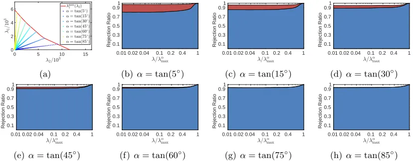
We perform experiments to evaluate TLFre on synthetic and real data sets in Sections 6.1.1 and 6.1.2, respectively. To measure the performance of TLFre, we compute the rejection ratios of (L1) and (L2), respectively. Specifically, letmbe the number of features that have
0 coefficients in the solution,G be the index set of groups that are discarded by (L1) andp be the number of inactive features that are detected by (L2). The rejection ratios of (L1) and (L2) are defined by r1 =
P
g∈Gng
m and r2 =
|p|
m, respectively. Moreover, we report the speedup gained by TLFre, i.e., the ratio of the running time of solver without screening to the running time of solver with TLFre.
To determine appropriate values ofα andλby cross validation or stability selection, we can run TLFre with as many parameter values as we need. Given a data set, for illustrative purposes only, we select seven values ofαfrom{tan(ψ) :ψ= 5◦,15◦,30◦,45◦,60◦,75◦,85◦}. Then, for each value ofα, we run TLFre along a sequence of 100 values ofλequally spaced on the logarithmic scale of λ/λαmax from 1 to 0.01. Thus, 700 pairs of parameter values of (λ, α) are sampled in total.
We usesgLeastRfrom the SLEP package (Liu et al., 2009) as the solver for SGL, which is one of the state-of-the-arts (Zhang et al., 2018b) [see Section G for a comparison between sgLeastR and another popular solver (Lin et al., 2014)].
For the non-screening case, we apply sgLeastR directly to solve SGL with different parameter values. We use zero as the initial point.
6.1.1. Simulation Studies
We perform experiments on two synthetic data sets that are commonly used in the literature (Tibshirani et al., 2012; Zou and Hastie, 2005). The true model is y = Xβ∗ + 0.01, ∼ N(0,1). We generate two data sets with 1000×160000 entries: Synthetic 1 and Synthetic 2. We randomly divide the 160000 features into 16000 groups. For Synthetic 1, the entries of the data matrixXare i.i.d. standard Gaussian with pairwise correlation zero, i.e., corr(xi,xi) = 0. For Synthetic 2, the entries of the data matrix X are drawn from
i.i.d. standard Gaussian with pairwise correlation 0.5|i−j|, i.e., corr(xi,xj) = 0.5|i−j|. To constructβ∗, we first randomly select γ1 percent of groups. Then, for each selected group,
we randomly select γ2 percent of features. The selected components of β∗ are populated
from a standard Gaussian and the remaining ones are set to 0. We set γ1 = γ2 = 10 for
Synthetic 1 andγ1=γ2 = 20 for Synthetic 2.
Fig. 1(a) and Fig. 2(a) show the plots of λmax1 (λ2) (see Corollary 12) and the sampled
parameter values of λ and α (recall thatλ1 =αλ and λ2 =λ). For the other figures, the
blue and red regions represent the rejection ratios of (L1) and (L2), respectively. We can
0 2 4 6 8 0
1 2
(a)
0.01 0.02 0.04 0.1 0.2 0.4 1 0.1 0.3 0.5 0.7 0.91 Rejection Ratio
(b) α= tan(5◦)
0.01 0.02 0.04 0.1 0.2 0.4 1 0.1 0.3 0.5 0.7 0.91 Rejection Ratio
(c)α= tan(15◦)
0.01 0.02 0.04 0.1 0.2 0.4 1 0.1 0.3 0.5 0.7 0.91 Rejection Ratio
(d) α= tan(30◦)
0.01 0.02 0.04 0.1 0.2 0.4 1 0.1 0.3 0.5 0.7 0.91 Rejection Ratio
(e) α= tan(45◦)
0.01 0.02 0.04 0.1 0.2 0.4 1 0.1 0.3 0.5 0.7 0.91 Rejection Ratio
(f)α= tan(60◦)
0.01 0.02 0.04 0.1 0.2 0.4 1 0.1 0.3 0.5 0.7 0.91 Rejection Ratio
(g)α= tan(75◦)
0.01 0.02 0.04 0.1 0.2 0.4 1 0.1 0.3 0.5 0.7 0.91 Rejection Ratio
(h) α= tan(85◦)
Figure 1: Rejection ratios of TLFre on the Synthetic 1 data set.
0 5 10 15 0
2 4 6
(a)
0.01 0.02 0.04 0.1 0.2 0.4 1 0.1 0.3 0.5 0.7 0.91 Rejection Ratio
(b) α= tan(5◦)
0.01 0.02 0.04 0.1 0.2 0.4 1 0.1 0.3 0.5 0.7 0.91 Rejection Ratio
(c)α= tan(15◦)
0.01 0.02 0.04 0.1 0.2 0.4 1 0.1 0.3 0.5 0.7 0.91 Rejection Ratio
(d) α= tan(30◦)
0.01 0.02 0.04 0.1 0.2 0.4 1 0.1 0.3 0.5 0.7 0.91 Rejection Ratio
(e) α= tan(45◦)
0.01 0.02 0.04 0.1 0.2 0.4 1 0.1 0.3 0.5 0.7 0.91 Rejection Ratio
(f)α= tan(60◦)
0.01 0.02 0.04 0.1 0.2 0.4 1 0.1 0.3 0.5 0.7 0.91 Rejection Ratio
(g)α= tan(75◦)
0.01 0.02 0.04 0.1 0.2 0.4 1 0.1 0.3 0.5 0.7 0.91 Rejection Ratio
(h) α= tan(85◦)
Figure 2: Rejection ratios of TLFre on the Synthetic 2 data set.
90% of inactive features can be detected. Moreover, we can observe that the first layer screening (L1) becomes more effective with a largerα. Intuitively, this is because the group Lasso penalty plays a more important role in enforcing the sparsity with a larger value of α (recall that λ1 = αλ). The top and middle parts of Table 1 indicate that the speedup
gained by TLFre is very significant (up to 80 times) and TLFre is very efficient. Compared to the running time of the solver without screening, the running time of TLFre is negligible. The running time of TLFre includes that of computingkXgk2, g= 1, . . . , G, which can be
efficiently computed by the power method (Halko et al., 2011). Indeed, this can be shared for TLFre with different parameter values.
6.1.2. Experiments on Real Data Sets
Table 1: Running time (in seconds) for solving SGL along a sequence of 100 tuning param-eter values ofλequally spaced on the logarithmic scale ofλ/λαmax from 1.0 to 0.01 by (a): the solver (Liu et al., 2009) without screening; (b): the solver combined with TLFre. The data sets are Synthetic 1 and Synthetic 2.
α tan(5◦) tan(15◦) tan(30◦) tan(45◦) tan(60◦) tan(75◦) tan(85◦)
Synthetic 1
solver 15555.28 16124.08 16106.24 16293.04 16426.44 16836.16 16862.36 TLFre 37.84 43.08 46.92 51.16 54.24 53.4 53.24 TLFre+solver 184.16 275.36 680.08 1196.04 1465.16 1629.96 1657.00
speedup 84.46 58.55 23.68 13.62 11.21 10.33 10.18
Synthetic 2
solver 15709.72 16615.16 16286.04 16826.48 16919.41 17178.08 17350.36 TLFre 41.72 47.28 54.08 54.72 59.08 58.56 60.12 TLFre+solver 328.52 906.72 1452.28 1702.61 1912.76 2181.23 2180.24
speedup 47.82 18.32 11.21 9.88 8.85 7.88 7.96
Table 2: Running time (in seconds) for solving SGL along a sequence of 100 tuning pa-rameter values ofλequally spaced on the logarithmic scale ofλ/λαmax from 1.0 to 0.01 by (a): the solver (Liu et al., 2009) without screening; (b): the solver com-bined with TLFre. We perform experiments on the ADNI data sets. The response vectors are GMV and WMV, respectively.
α tan(5◦) tan(15◦) tan(30◦) tan(45◦) tan(60◦) tan(75◦) tan(85◦)
ADNI+GMV
solver 30652.56 30755.63 30838.29 31096.10 30850.78 30728.27 30572.35 TLFre 64.08 64.56 64.96 65.00 64.89 65.17 65.05 TLFre+solver 372.04 383.17 386.80 402.72 391.63 385.98 382.62
speedup 82.39 80.27 79.73 77.22 78.78 79.61 79.90
ADNI+WMV
solver 29751.27 29823.15 29927.52 30078.62 30115.89 29927.58 29896.77 TLFre 62.91 63.33 63.39 63.99 64.13 64.31 64.36 TLFre+solver 363.43 364.78 386.15 393.03 395.87 400.11 399.48
speedup 81.86 81.76 77.50 76.53 76.08 74.80 74.84
Table 3: Running time (in seconds) for solving SGL along a sequence of 100 tuning param-eter values ofλequally spaced on the logarithmic scale ofλ/λαmax from 1.0 to 0.01 by (a): the solver (Liu et al., 2009) without screening; (b): the solver combined with TLFre. We perform experiments on the news20.binary data sets.
α tan(5◦) tan(15◦) tan(30◦) tan(45◦) tan(60◦) tan(75◦) tan(85◦)
news20.binary
solver 1233401.05 1231570.22 1277630.92 1299353.68 1292879.86 1216554.09 1347890.85 TLFre 350.51 337.75 332.01 346.98 352.78 353.52 362.43 TLFre+solver 1434.49 1465.37 1539.37 1598.87 1608.90 1659.78 1709.35
0 50 100 150 0 50 100 λ2 λ1 λmax 1 (λ2)
α= tan(5◦)
α= tan(15◦)
α= tan(30◦)
α= tan(45◦)
α= tan(60◦)
α= tan(75◦)
α= tan(85◦)
(a)
0.01 0.02 0.04 0.1 0.2 0.4 1 0.1
0.3 0.5 0.7 0.91
λ/λα
max
Rejection Ratio
(b) α= tan(5◦)
0.01 0.02 0.04 0.1 0.2 0.4 1 0.1
0.3 0.5 0.7 0.91
λ/λα
max
Rejection Ratio
(c)α= tan(15◦)
0.01 0.02 0.04 0.1 0.2 0.4 1 0.1
0.3 0.5 0.7 0.91
λ/λα
max
Rejection Ratio
(d) α= tan(30◦)
0.01 0.02 0.04 0.1 0.2 0.4 1 0.1
0.3 0.5 0.7 0.91
λ/λα
max
Rejection Ratio
(e) α= tan(45◦)
0.01 0.02 0.04 0.1 0.2 0.4 1 0.1
0.3 0.5 0.7 0.91
λ/λα
max
Rejection Ratio
(f)α= tan(60◦)
0.01 0.02 0.04 0.1 0.2 0.4 1 0.1
0.3 0.5 0.7 0.91
λ/λα
max
Rejection Ratio
(g)α= tan(75◦)
0.01 0.02 0.04 0.1 0.2 0.4 1 0.1
0.3 0.5 0.7 0.91
λ/λα
max
Rejection Ratio
(h) α= tan(85◦)
Figure 3: Rejection ratios of TLFre on the ADNI data set with grey matter volume as response.
0 50 100 150 0 50 100 λ2 λ1 λmax 1 (λ2)
α= tan(5◦)
α= tan(15◦)
α= tan(30◦)
α= tan(45◦)
α= tan(60◦)
α= tan(75◦)
α= tan(85◦)
(a)
0.01 0.02 0.04 0.1 0.2 0.4 1 0.1
0.3 0.5 0.7 0.91
λ/λα
max
Rejection Ratio
(b) α= tan(5◦)
0.01 0.02 0.04 0.1 0.2 0.4 1 0.1
0.3 0.5 0.7 0.91
λ/λα
max
Rejection Ratio
(c)α= tan(15◦)
0.01 0.02 0.04 0.1 0.2 0.4 1 0.1
0.3 0.5 0.7 0.91
λ/λα
max
Rejection Ratio
(d) α= tan(30◦)
0.01 0.02 0.04 0.1 0.2 0.4 1 0.1
0.3 0.5 0.7 0.91
λ/λα
max
Rejection Ratio
(e) α= tan(45◦)
0.01 0.02 0.04 0.1 0.2 0.4 1 0.1
0.3 0.5 0.7 0.91
λ/λα
max
Rejection Ratio
(f)α= tan(60◦)
0.01 0.02 0.04 0.1 0.2 0.4 1 0.1
0.3 0.5 0.7 0.91
λ/λα
max
Rejection Ratio
(g)α= tan(75◦)
0.01 0.02 0.04 0.1 0.2 0.4 1 0.1
0.3 0.5 0.7 0.91
λ/λα
max
Rejection Ratio
(h) α= tan(85◦)
Figure 4: Rejection ratios of TLFre on the ADNI data set with white matter volume as response.
ADNIThe data matrix of the ADNI data set consists of 747 samples with 426040 single nucleotide polymorphisms (SNPs), which are divided into 94765 groups. The response vectors are the grey matter volume (GMV) and white matter volume (WMV), respectively.
news20.binary The news20.binary data set consists of 19996 samples with 1355191 features, which are divided into 67760 groups. The entries of the response vectors are the labels of the corresponding samples, which are 1 or−1.
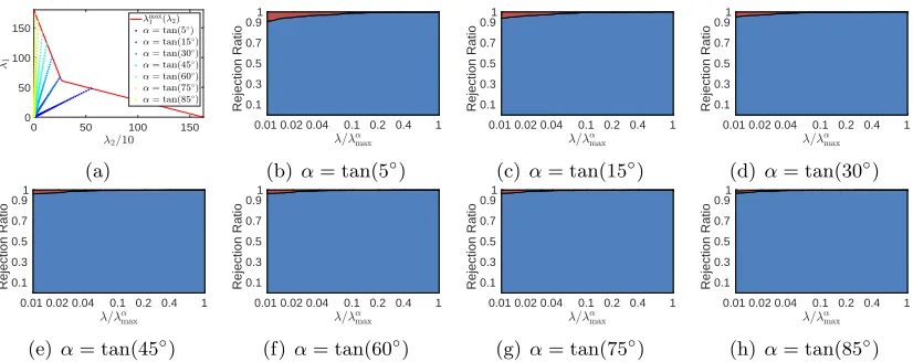
Fig. 3(a), Fig. 4(a), and Fig. 5(a) show the plots ofλmax1 (λ2) (see Corollary 12) and the
sampled parameter values ofαand λ. The other figures present the rejection ratios of (L1) and (L2) by blue and red regions, respectively. We can see that almost all of the inactive
groups/features are discarded by TLFre. The rejection ratios ofr1+r2are very close to 1 in
0 50 100 150 0
50 100 150
(a)
0.01 0.02 0.04 0.1 0.2 0.4 1 0.1
0.3 0.5 0.7 0.91
Rejection Ratio
(b) α= tan(5◦)
0.01 0.02 0.04 0.1 0.2 0.4 1 0.1
0.3 0.5 0.7 0.91
Rejection Ratio
(c)α= tan(15◦)
0.01 0.02 0.04 0.1 0.2 0.4 1 0.1
0.3 0.5 0.7 0.91
Rejection Ratio
(d) α= tan(30◦)
0.01 0.02 0.04 0.1 0.2 0.4 1 0.1
0.3 0.5 0.7 0.91
Rejection Ratio
(e) α= tan(45◦)
0.01 0.02 0.04 0.1 0.2 0.4 1 0.1
0.3 0.5 0.7 0.91
Rejection Ratio
(f)α= tan(60◦)
0.01 0.02 0.04 0.1 0.2 0.4 1 0.1
0.3 0.5 0.7 0.91
Rejection Ratio
(g)α= tan(75◦)
0.01 0.02 0.04 0.1 0.2 0.4 1 0.1
0.3 0.5 0.7 0.91
Rejection Ratio
(h) α= tan(85◦)
Figure 5: Rejection ratios of TLFre on the news20.binary data set.
each value ofαon the ADNI and news20.binary data set, respectively. However, combined with TLFre, the solver needs only 6∼8 minutes and 24∼29 minutes, respectively. Moreover, we can observe that the computational cost of TLFre is negligible compared to that of the solver without screening. This demonstrates the efficiency of TLFre.
6.2. DPC for Nonnegative Lasso
In this experiment, we evaluate the performance of DPC on two synthetic data sets and six real data sets. We integrate DPC with the solver, nnLeastR, (Liu et al., 2009) to solve the nonnegative Lasso problem along a sequence of 100 parameter values ofλequally spaced on the logarithmic scale of λ/λmax from 1.0 to 0.01. The two synthetic data sets are the same
as the ones we used in Section 6.1.1. To construct β∗, we first randomly select 10 percent of features. The corresponding components of β∗ are populated from a standard Gaussian and the remaining ones are set to 0.
We usennLeastRfrom the SLEP package (Liu et al., 2009) as the solver for nonnegative Lasso, which is one of the state-of-the-arts [see Section G for a comparison between nnLeastR and another popular solver (Lin et al., 2014)].
For the non-screening case, we apply nnLeastR directly to solve SGL with different parameter values. We use zero as the initial point.
We list the six real data sets and the corresponding experimental settings as follows.
Breast Cancer data set (West et al., 2001; Shevade and Keerthi, 2003): this data set contains 7129 gene expression values of 44 tumor samples (thus the data matrixX is of 44×7129). The response vector y∈ {1,−1}44 contains the binary label of each sample.
Leukemia data set (Armstrong et al., 2002): this data set contains 11225 gene ex-pression values of 52 samples (X ∈R52×11225). The response vector y contains the binary
label of each sample.
Prostate Cancer data set (Petricoin et al., 2002): this data set contains 15154 mea-surements of 132 patients (X ∈ R132×15154). By protein mass spectrometry, the features
constituent proteins in the blood. The response vector y contains the binary label of each sample.
PIE face image data set (Sim et al., 2003; Cai et al., 2007): this data set contains 11554 gray face images (each has 32×32 pixels) of 68 people, taken under different poses, illumination conditions and expressions. In each trial, we first randomly pick an image as the response y ∈ R1024, and then use the remaining images to form the data matrix X∈R1024×11553. We run 100 trials and report the average performance of DPC.
MNIST handwritten digit data set(Lecun et al., 1998): this data set contains grey images of scanned handwritten digits (each has 28×28 pixels). The training and test sets contain 60,000 and 10,000 images, respectively. We first randomly select 5000 images for each digit from the training set and get a data matrixX∈R784×50000. Then, in each trial,
we randomly select an image from the testing set as the response y ∈ R784. We run 100
trials and report the average performance of the screening rules.
Street View House Number (SVHN) data set (Netzer et al., 2001): this data set contains color images of street view house numbers (each has 32×32 pixels), including 73257 images for training and 26032 for testing. In each trial, we first randomly select an image as the responsey∈R3072, and then use the remaining ones to form the data matrix X∈R3072×99288. We run 20 trials and report the average performance.
0.01 0.02 0.04 0.1 0.2 0.4 1 0.1 0.3 0.5 0.7 0.9 1 Rejection Ratio
(a) Synthetic 1
0.01 0.02 0.04 0.1 0.2 0.4 1 0.1 0.3 0.5 0.7 0.9 1 Rejection Ratio
(b) Synthetic 2
0.010 0.02 0.04 0.1 0.2 0.4 1
0.2 0.4 0.6 0.8 1
λ/λmax
Rejection Ratio
(c) Breast Cancer
0.010 0.02 0.04 0.1 0.2 0.4 1
0.2 0.4 0.6 0.8 1
λ/λmax
Rejection Ratio
(d) Leukemia
0.010 0.02 0.04 0.1 0.2 0.4 1
0.2 0.4 0.6 0.8 1
λ/λ max
Rejection Ratio
(e) Prostate Cancer
0.010 0.02 0.04 0.1 0.2 0.4 1
0.2 0.4 0.6 0.8 1
λ/λ max
Rejection Ratio
(f) PIE
0.010 0.02 0.04 0.1 0.2 0.4 1
0.2 0.4 0.6 0.8 1
λ/λ max
Rejection Ratio
(g) MNIST
0.010 0.02 0.04 0.1 0.2 0.4 1
0.2 0.4 0.6 0.8 1
λ/λ max
Rejection Ratio
(h) SVHN
Figure 6: Rejection ratios of DPC on eight data sets.
Table 4: Running time (in seconds) for solving nonnegative Lasso along a sequence of 100 tuning parameter values of λ equally spaced on the logarithmic scale of λ/λmax
from 1.0 to 0.01 by (a): the solver (Liu et al., 2009) without screening; (b): the solver combined with DPC.
Synthetic 1 Synthetic 2 Breast Cancer Leukemia Prostate Cancer PIE MNIST SVHN solver 13140.84 13853.84 23.40 34.04 187.82 674.04 3000.69 24761.07
DPC 3.08 3.59 0.03 0.06 0.23 1.16 3.53 30.59
DPC+solver 61.56 69.52 2.18 3.37 6.37 5.01 9.31 104.93