Correlation method for measuring the largest Lyapunov exponent in optical fields

(1)

Correlation method for measuring the largest

Lyapunov exponent in optical fields

Gavrylyak M.S., Maksimyak A.P. and Maksimyak P.P.

Department of Correlation Optics, Yuri Fedkovych Chernivtsi National University, 2 Kotsyubinsky St., 58012 Chernivtsi, Ukraine

e-mail: [email protected] Received:25.03.2008

Abstract

We propose an analog interference method for measuring the largest Lyapunov exponent for the optical fields generated by scattering objects and media. The method is further developed to make a device for high-speed real-time measurements of transverse correlation function of the optical fields.

Keywords: space-time chaos, the largest Lyapunov exponent, transverse correlation function, nematic liquid crystal, interference method. PACS: 42.25.Hz, 42.25.Fx

UDC: 535.36, 535.41

1. Introduction

The studies of spatial complexity of optical fields have started about twenty years ago [1– 3]. The correlation, spectral and other methods commonly used to analyze random fields usually give little or no information on the nature of system that generates those fields. For instance, one cannot determine whether the field is generated by a random object or a deterministic, though complex enough, system.

Any optical scatter or object may be considered as a system that can generate both time and space-time chaos [4, 5]. For a time-independent case, a notion of optical field dimension may be introduced by analogy with the time-dependent case [6, 7]. For dynamic systems [8, 9], sensitivity to initial conditions is quantified by the Lyapunov exponent [10]. Consider, for example, two trajectories with nearby initial conditions on an attracting manifold. When the attractor is chaotic, the trajectories diverge, on average, at an exponential rate characterized by the largest Lyapunov exponent [11]. The problem of characterizing the evolution of infinitesimal perturbations becomes even more complex for spatially extended systems.

(2)

Ukr. J. Phys. Opt. 2008, V9, №2 120

2. Calculations of the largest Lyapunov exponent

The Lyapunov exponent characterizes the average velocity of exponential divergence of close phase trajectories. If d0 is an initial distance between two initial points of the phase trajectories, the distance between the trajectories, coming off these points, will depend on time t as follows:

t

e

d

t

d

λ

0

)

(

=

. (1)

The quantity λ is called as the Lyapunov exponent [12]. Each dynamic system is characterized by entire spectrum of Lyapunov exponents λи (и = 1, 2, …, n), where n

denotes the number of differential equations which are necessary for description of the system. The positive Lyapunov exponent obtained from the experimental data based on observing dynamic systems can be a proof for chaos existing in those systems. Generally speaking, a chaotic system is characterized by divergence of the phase trajectories in some similar directions and, simultaneously, their convergence in the other ones, i.e. there are both positive and negative Lyapunov exponents for the given chaotic system. The sum of all the indices can be negative, i.e. the degree of trajectory convergence can exceed that of divergence. If this condition is not satisfied, the dynamic system is instable and its behaviour is easily recognized. Thus, in most cases, it is sufficient to calculate the largest Lyapunov exponent only. The positive value of the latter indicates a possibility for chaos existing in the system, and the value of this index characterizes intensity of the chaos.

Most of the algorithms that have so far been applied for calculating the largest Lyapunov exponent manifest some disadvantages. As a rule, they require a great amount of experimental data. Moreover, the programs needed for realization of the algorithms are comparatively complex and many time-consuming calculations are involved [8]. Using the theoretical results described in the work [13], we have elaborated the algorithm and the program for calculating the largest Lyapunov exponent. They turn out to be free of disadvantages mentioned above.

The first algorithmic step suggested by us consists in reconstructing the phase trajectory. It is represented in the form of a matrix X, each column of which is a vector in the phase space,

T M 2

1 X ... X ]

X [

X= ,

where X_i denotes the state of the system at the point of time i. For the series of N

measurements

{

x

1

,

x

2

,..,

x

N

}

, any

X

is defined as follows:

] x

... x x [

X_i = _i _i₊_J _i₊₍_m₋₁₎_J ,

where J is the time delay (the so-called reconstruction delay) and m the embedding dimension. Thus, the quantity X represents some M×m matrix, while the constants m,

(3)

with

D

being the Hausdorff measure of the original system. The limiting m value is referred to as the embedding dimension of the system. However, the method described here enables one to derive the correct result at smaller m values. The reconstruction delay is chosen as being equal to the time, for which the autocorrelation function decreases as 1 – 1/е from its initial value.

After reconstructing the phase trajectory with the above algorithm, a search of the nearest “neighbour” for each trajectory point is expected, where the nearest “neighbour” is regarded as a point

X

_j with the minimum distance (0)d_j from the basic point

X

_j:

(0) m in || ||

j

j _X j j

d = X −X

_.₍₂₎

Following the work by Rosenstein et al. [13], one can find that the couple of “neighbour” points diverges exponentially in some time period ∆t:

) (

1

)

(

i t

j

i

C

e

d

≈

λ ⋅∆ _,₍₃₎

where λ1 means the largest Lyapunov exponent and

C

j the initial separation

( ( ) 1(i t)

j j

d i _≈C eλ ∆ _). _{By taking logarithm on both sides of Eq.}_{(3), we obtain}

1

ln ( ) lnd i_j ≈ C_j+λ(i t∆ ). Eq. (3) represents a set of approximately parallel lines (for j

= 1, 2, ... , M), each with a slope roughly proportional to

λ

₁.

The largest Lyapunov exponent might be easily and accurately calculated using the least-square fit to the “average” line defined by

1

( ) ln ( )j

y i d i

t

= 〈 〉

∆ , (4)

where <…> means the value averaged for all j.

The results for the Henon’s mapping are demonstrated in Fig. 1. The diagram inclination has been calculated with the aid of the least-square technique. We have obtained the value λ1 = 0.403 that almost corresponds to the theoretical one (λ1 = 0.418).

(4)

Ukr. J. Phys. Opt. 2008, V9, №2 122

3. Interference method for measuring the largest Lyapunov exponent for the field intensity

For spatially inhomogeneous fields, such as a speckle field, the constructed dynamic system will have the same dimension as the original system for

m

>

2 D

+

1

[15]. In order to calculate the largest Lyapunov exponent for a single generalized coordinate, namely for the intensity

I

( )

r

of the object field, we construct the dynamic systems, so that

( )

_[

_]

1 1

, ,...,

m

i i i i m

I = I I+ I+ − , (5)

where I_i are the field intensities at the points x_i.

The numerical “distances” from the ith to jth points are given by

( )

[

(

) (

)

2

(

)

2

]

1 2

1 1 2 / ) (

_...

m j m i j i j i m j m

i

I

−

=

−

+

₊

−

₊

+

₊

−

₊ . (6)

For a single generalized coordinate, the field intensity I

( )

r , we construct the relation given by Eq. (4), whose slope is proportional to

λ

₁.

Thus, the procedure by Rosenstein et al. [13] discussed in Sec. 2 may be used for evaluation of the largest Lyapunov exponent

λ

₁. However, direct application of this procedure to real physical systems with high embedding dimensions is difficult, since it requires a large number of sampling points.

To bypass the difficulties associated with digital processing, we suggest performing some operations in the analog mode. The Lyapunov exponent

λ

₁ appears to be closely related to some correlation characteristics of optical fields, particularly the structure function [16]

2

1 2 1 2

( , ) ( ) ( )

I

D r r = I r −I r . (7)

For locally uniform and isotropic fields, the intensity structure function is linked to the intensity correlation function,I⊥

( )

ρ , through the relation

(

)

I

( )

ρ

[

I

( )

I

( )

ρ

]

I r r D

D ₁, ₂ = =2Ψ 0 −Ψ , (8)

where ΨI

( )

ρ and ΨI

( )

0 are the transverse intensity correlation functions for ρ= r1−r2 and

ρ

=

0

, respectively.

Let us consider the numerical “distances” given by Eq. (6) and introduce the separation between two points in the m-dimensional space,

( ) ( ) 1

(

)

1/2

0 2       − = −

∑

− = + + m k k j k i m j m

i I I I

I . (9)

(5)

Now we present our interference technique for measuring the largest Lyapunov exponent in optical fields for the case of intensity distribution in nematic liquid crystal cell (the white-light image, see Fig. 2).

Fig. 2. Optical field for the intensity distribution in nematic liquid crystal cell (white-light image).

A nematic liquid crystal E7 is sandwiched between two glass substrates. The cell gap is maintained by a 7 µm-thick spacer film. Electric field is applied to the liquid crystal cell using transparent ITO electrodes deposited on internal surfaces of the glass substrates. Sinusoidal electric field (25 V and 2000 Hz) is applied to the composite cell. In this case chaotic space-time fluctuations are present in the system.

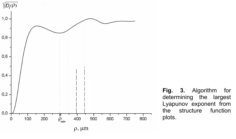
Fig. 3 shows the algorithm for calculating the Lyapunov exponent

λ

₁ from the plot of the structure function D_I

( )

ρ , which has been determined for the intensity distribution displayed in Fig. 2.

(6)

Ukr. J. Phys. Opt. 2008, V9, №2 124

First we find the quantity

ρ

_⊥ equal to the lag where the structure function drops to 1/e from its initial value. For

ρ

>

ρ

_⊥ we locate the nearest neighbourof each point on the trajectory, for which Eq. (2) is true. This transverse displacement in Fig. 3 corresponds to

ρ

min and is greater than the average period of spatial fluctuations of the intensity field.

The distance between the trajectories in the m-dimensional space,

( ) ( ) 1

(

)

1 2

0 2 /









₋

=

−

∑

− = + + m k k j k i m j m

i

I

, will be given by d(1)= DI(ρ) for different

values l = i− j = ρ /δr. Then the largest Lyapunov exponent

λ

₁ can be easily found

from the slopes of dependences of l versus ( ) ( _min) 1 ln D (l)

r y l y _I δ ρ

ρ− =

= . In

particular, for locally uniform and isotropic optical fields we have )

( ln ) (

ln DI ρ = DI ρ .

The embedding dimension, i.e. the value m, is taken to be very large in order to approximate the structure function (9) with adequate accuracy. In addition, the structure function has the same form for large data arrays, irrespective of the origin of ρ. Consequently, a single D_I

( )

ρ curve would be sufficient for calculating the largest Lyapunov exponent

λ

₁ for the field intensity I

( )

r .

The curve DI

( )

ρ could be obtained from either measured or calculated functions

( )

[

_ρ

]

1/2

I

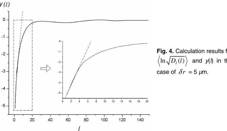
D . Then the curve y(l)= f(ln D_I(l)) is constructed for the number of points used in calculating the structure function (it is equal to m=N/2 – see Fig. 4). The largest Lyapunov exponent of thus constructed dynamic systems (5) for the field intensity

( )

r

I (see Fig. 2), which has been calculated using the procedure of Rosenstein et al.[13] (

λ

₁ = 0.187), agrees well with that obtained on the basis of commonly used method (

λ

₁ = 0.191). However, the processing time has been reduced by about two orders of magnitude.

The intensity structure function may be evaluated by measuring the local field intensities using the computer processing of the data and Eq. (7). Another possibility is to measure the transverse intensity correlation function using an intensity correlator and then substitute the data into Eq. (8). The function could also be evaluated by measuring the field correlation function with a shearing interferometer, subsequently determining the intensity structure function

D

_I

( )

ρ

and employing the relation [15]

[

2

]

) ( 1 ) 0 ( 8 )

(

ρ

= Γ_⊥ −Γ_⊥

ρ

I

D , (10)

(7)

Fig. 4. Calculation results for ln D l_I( ) and y(l) in the case of δr = 5 µm.

Fig. 5 illustrates the experimental setup for measuring the largest Lyapunov exponent for the intensity of coherent optical fields.

Fig. 5. Optical arrangement for measuring the correlation exponent: He-Ne, laser; T, telescope; S, sample; SI, shearing interferometer; O, objective lens; FD, field-of-view diaphragm; PD, photodetector; ADC, analog-to-digital converter; PC, personal computer.

(8)

Ukr. J. Phys. Opt. 2008, V9, №2 126

4. Conclusion

In summary, we have proposed the interference approach aimed at derivation of the largest Lyapunov exponent for the coherent chaotic optical fields. For this aim we have applied high-speed real-time correlation techniques. The largest Lyapunov exponent for the field intensity calculated using our procedure has appeared to be in good agreement with that obtained by the commonly adopted method.

References

1. Harrison R. G., Firth W. J. and Al-Saidi I. A. Instabilities and routes to chaos in passive all-optical resonators containing molecular gases. Instabilities and Chaos in Quantum Optics, Arecchi F. T. and Harrison R. G., eds., Berlin: Springer Verlag (1987), 201–236.

2. Arecchi F T, Boccaletti S, Giacomelli G, Puccioni G P, Ramazza P L and Residori S, 1992. Patterns, space-time chaos and topological defects in nonlinear optics. Physica D 61: 25–39.

3. Asakura T. and Uozumi J. Fractal Optics. Sapporo: Hokkaido Univ. Press (1995). 4. Toronov V Y, Zhang X and Webb A G, 2007. A spatial and temporal comparison of

hemodynamic signals measured using optical and functional magnetic resonance imaging during activation in human primary visual cortex. NeuroImage 34: 1136– 1148.

5. Barré J and Dauxois T, 2001. Lyapunov exponents as a dynamical indicator of a phase transition. Europhys. Lett. 55: 164–170.

6. Ebisawa S and Komatsu S, 2007. Message encoding and decoding using an asynchronous chaotic laser diode transmitter–receiver array. Appl. Opt. 46: 4386– 4396.

7. Politi A, Ginelli F, Yanchuk S and Maistrenko Y, 2006. From synchronization to Lyapunov exponents and back. Physica D 224: 90–101.

8. Eckmann J-P and Ruelle D, 1985. Ergodic theory of chaos and strange attractors. Rev. Mod. Phys. 57: 617–656.

9. Farmer J D and Sidorowich J J, 1987. Predicting chaotic time series. Phys. Rev. Lett. 59: 845–848.

10. Sano M and Sawada Y, 1985. Measurement of the Lyapunov spectrum from a chaotic time series. Phys. Rev. Lett. 55: 1082–1085.

11. Wolf A., Swift J B, Swinney H L and Vastano J A, 1985. Determining Lyapunov exponents from a time series. Physica D 16: 285–317.

12. Neumark Yu. I. and Landa P. S., Stochastic and Chaotic Fluctuations. Moscow: Nauka (1987).

(9)

14. Takens F, 1981. Detecting strange attractors in turbulence. Lect. Notes in Math. 898: 366–381.

15. Angelsky O V, Maksimyak P P and Perun T O, 1993. Dimensionality in optical fields and signals. Appl. Opt. 32: 6066–6071.

16. Rytov S. M. , Kravtsov Yu. A. and Tatarsky V. I. Principles of Statistical Radio-physics. Berlin: Springer (1989).