Nonlinear optimized Fast Locking PLLs Using Genetic Algorithm

Nonlinear Optimized Fast Locking PLL; using Genetic

Algorithm

M. Zabihi* and H. Miar-Naimi*

Abstract: This paper presents a novel approach to obtain fast locking PLL by embedding a nonlinear element in the loop of PLL. The nonlinear element has a general parametric Taylor expansion. Using genetic algorithm (GA) we try to optimize the nonlinear element parameters. Embedding optimized nonlinear element in the loop shows enhancements in speed and stability of PLL. To evaluate the performance of the proposed structure, various tests performed and results compared with standard phase locked loop. The tests and results show the superior performance of the proposed PLL.

Keywords: PLL, Genetic Algorithm, Nonlinear Element, Fast lock.

1 Introduction1

Phase locked loops have wide applications in communication circuits such as radio frequency transmitters, wireless communications, optical receivers and etc. They also serve different systems as a main building block. As example, systems like frequency modulators, frequency synthesizers, clock and data recovery circuits can be addressed [1-10]. The performance of PLL is critical for the above applications so that high performance PLLs was the subject of many researches in the field of electronics and communication system design. The most important performance measure of PLLs is the capture range and the speed of locking. Fast locking PLLs provide the mentioned systems to work in higher speeds. There are some works on speeding up the lock process. In [8] using an adaptive system, the bandwidth of loop filter is controlled based on the lock condition. When the loop is far from locked condition a large value for bandwidth is chosen that causes higher loop gain and consequently smaller rise time. To avoid large overshoots the bandwidth is reduced when the loop closes to locked condition. It is clear that this method requires an efficient subsystem to measure the distance to lock condition. The paper mentioned nothing about the detail of the subsystem. In another approach a nonlinear element is embedded to the loop [9]. Nonlinear element has a profile implementing somehow the idea of [10]. To perform this, the slop of transfer function is chosen inconstant and varies for different values of its input.

Iranian Journal of Electrical & Electronic Engineering, 2009. Paper first received 17 Sep. 2009 and in revised form 16 Nov. 2009. * The Authors are with the Department of Electrical and Computer Engineering, Babol University of Technology, Babol, Iran.

E-mails: [email protected], [email protected].

Some significant questions arise here such as: what is the best or optimal nonlinear element for the loop? Is there any straightforward way to find optimal nonlinear element analytically or numerically. This paper introduces a novel method that one can find the best nonlinear element using genetic algorithm. Indeed the algorithm searches in mathematic functions space. The rest of paper is as follows: in section 2 the dynamic of a type I PLL is introduced and the tradeoff between overshoot and rise time is addressed. Section 3 deals with Genetic Algorithm method for optimization of the nonlinear element parameters. This method has a major role in proposed PLL. Section 4 introduces the new nonlinear PLL and related differential equations and also the related genetic algorithm finding optimal solutions. In this section, the nonlinear element is optimized using Genetic Algorithm. Finally the conclusion is given in section 5.

2 Dynamic of Phase Locked Loop; A Brief Review A phase locked loop is a system which generate a periodical output in phase to an arbitrary periodical input. A conceptual or mathematical phase locked loop has a general block diagram as shown in Fig. 1. This block diagram represents the dynamics governing on the PLL.

In Fig. 1 the first block is phase detector, PD, that measures the phase difference between input and output waveforms. The second block is a voltage controlled oscillator, VCO that generates a periodical output with a frequency depending to the phase difference. The philosophy of above block diagrams can be found in text books [1-2]. In Fig. 1, ψinand ψout are the input and output phases defined as ψ_in( )t =ω_it and based on

the definition of VCO:

1

( )

out t outt ct kvcov dt

ψ =ω =ω +

∫

control voltage of VCO and is proportional to phase difference by a coefficient ofKPD, and ωc is the central frequency of VCO. To find the dynamic of the above system, we can write:

(1)

∫

− o e it ct kvcov dt

i ψ ψ ω ω 1

ψ (2) e PD o i PD vco c i

e ω ω k v v k ψ ψ k ψ

ψ& = − − 1, 1= ( − )=

(3) e PD vco c i

e ω ω k k ψ

ψ& = − −

Equation (1) is a first order differential equation describing the behavior of the system. As a direct consequence of Eq. (1), when the system reaches to a steady state (locked condition) we have ψ&_e=0

resulting in ωout =ωi and

i c e

vco PD

k k

ω ω

ψ = − . The equation

above can be simply rewritten in term of control voltage. The step response of the system above has an

exponential form with time constant of 1 vco PD

k k , larger loop gain, higher speed in locking process. The above differential equation was written in term of total phase of input an output, without loss of generality above equations can be represented in term of excess phase defined as ψex in, =ψi−ω ψct, ex out, =ψo−ωctwithout any changes in equations.

In practical type-I PLLs phase detectors usually require a low pass filter as shown in Fig. 2 [1-2]. So to have a more general and practical model, we consider the dynamical model of Fig. 2 for a PLL.

The equations governing on the model above can be written as follows (ψ ψ_in, _outare excess phases).

PD VCO 1 v out

ψ

ψ

Fig. 1 Block diagram of a conceptual PLL

Fig. 2 Dynamical model of a second order type-I PLL

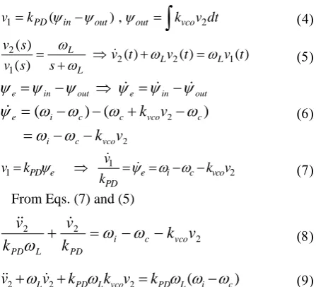
From Eqs. (7) and (5)

Equation (9) is the dynamical behavior of second order PLL.

This dynamic in term of input excess phase and output excess phase can be described by closed loop transfer function of Eq. (10).

whereξ and ωn are as Eq. (11).

The transfer function of Eq. (10) has two poles as shown in Eq. (12). The root locus of Eq. (10) is shown in Fig. 3. For ξ>1 both poles are real. By decreasing

ξ equivalently increasing of loop gain the poles becomes complex.

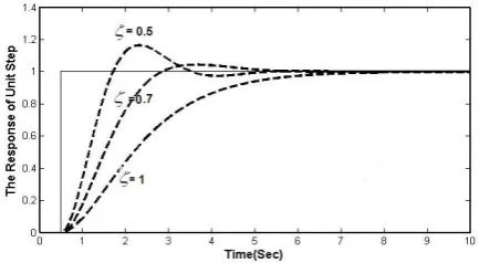
The Fig. 4 shows the step response of the system for different value of ξ.

As Fig. 4 shows, there is a tradeoff between rise time and overshoot where small rise time results in big overshoot. So controllingξ, one can not reach to a very fast locking system.

(4)

1 PD( in out) , out vco 2

v =k ψ −ψ ψ =

∫

(5)

2

2 2 1

1 ( ) ( ) ( ) ( ) ( ) L L L L v s

v t v t v t

v s s

ω _{ω ω}

ω = ⇒ + = + & (6) out in e out in

e

ψ

ψ

ψ

ψ

ψ

ψ

2 2 ) ( ) ( v k v k vco c i c vco c c i e − − = − + − − =

ω

ω

ω

ω

ω

ω

ψ

1 PD e e i c vco 2

PD

v

v k k v

k

ψ ψ ω ω

= ⇒ & = & = − −

(8) 2 2 2

v

k

k

v

k

v

−

−

=

+

ω

ω

ω

&

&&

2 Lv kPD Lkvcov kPD L i c

v_&& +

ω

ω

ω

ω

ω

(10) 2 2 2 ( ) 2 n n n H s s s ω ξω ω = + + (11) 1 , 2 LPF n VCO PD LPF

VCO PD

K K

K K

ω

ω = ω ζ =

(12)

2 1,2 n( 1)

s =ω ξ± ξ −

Fig. 3 The root locus of transfer function of Eq. (10)

Settling time, rise time and overshoot of the system above are derived as Eqs. (13) to (15) from [1, 2].

As mentioned above there are a tradeoff that prevents ideal step response of system. To break down this tradeoff we embed a parametrical nonlinear element in the loop and try to tune the parameters for best step response.

3 Genetic Algorithm; A Brief Review

Genetic Algorithms (GAs) are adaptive heuristic search algorithm based on the evolutionary ideas of natural selection and genetics. The basic hypothesis of this algorithm is that the congenital patterns in each generation transmit with gens to next generation The initial parameters are selected randomly and form the initial population [11-15]. The population evolves from The Genetic Algorithm process is explained as follows:

1. Initial parameters definitions: Such as number of pop1ulation, number of generation, mutation probability, crossover probability and chromosome length.

2. Producing Initial population: Initial population is generated randomly from search space.

3. Evaluation of each chromosome: each chromosome of population is assigned a value as fitness, based on objective function.

4. Testing stop condition: If the end condition such as number of generation is satisfied, the algorithm stops and returns the best solution in current population.

5. Producing new population: In this state a new population is created by repeating following steps until the new population is complete. According to the chromosome evaluation, two chromosomes are selected from the population as parents and genetic operators are applied on them. Crossover mixes two parent

chromosomes and creates new offspring with probability of Pc. Mutation operator changes random bit from 1 to 0 or vice versa with a small probability of mutation (Pm) which is much smaller than Pc.

6. Replacing populations: in this state, current population is replaced with the new population.

7. Loop: Go to step 2 and repeat [11, 13].

4 Proposed Nonlinear PLL

4.1 System Overview

In proposed phase locked loop a nonlinear element is embedded into the loop of PLL, hopping obtain faster transient. Shown in Fig. 5 is the proposed PLL structure, which is almost the same as [9]. In this method we fined the optimal nonlinear element aiming best speed. To obtain the equations governing the system, considering Fig. 5, we can write Eqs. (16)-(22).

Equation (21) is the second order nonlinear equation describing the system. To evaluate the locking speed in locked conditions the related differential equation is as Eq. (22).

We evaluate the response for a step in input phase and hope to have similar step in output phase in an ideal condition. For generality, the nonlinear element can be

considered as

0

( ) N

n n n

f v a v

=

=

∑

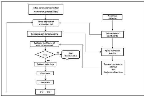
approximating every desired nonlinear function. For finding appropriate coefficients of f(v), at first N, the order of polynomial should be specified. In fact N is number of gens in this optimization problem. Therefore we have a optimization problem with N _parameters which can be solve by Genetic Algorithm. This process is shown in Fig. 6.

Fig. 4 the step response of system for different values ofξ

(13)

4.8 1

,

2

s n L

n

t ξω ω

ξω

= =

(14)

1 2

cos 1 r

n

t π ξ

ω ξ

− − =

−

(15)

2

1 ζ

πζ

− −

=

e

M

(16)

1 PD( in out)

v =k ψ −ψ

(17)

2 L 2 L 1

v& +ω v =ω v

(18)

3 ( 2)

out kvcov kvcof v

ψ& = =

(19)

1 PD( in out) PD( i c vco ( ))2

v_& =k ψ& −ψ& =k ω ω− −k f v

(20) ))

(

( ₂

2

2 _{v k k f v}

v

vco c i PD L

− − =

+ ω ω

ω&& &

(21)

2 L 2 PD L vco ( )2 PD L( i c)

v +ω v +k ω k f v =k ω ω ω−

&& &

(22)

2 L 2 PD L vco ( 2) 0

v&& +ω v& +k ω k f v =

PD

LPF LPF

s

ω

ω

+

f

(

v

)

VCO

v

v

v

out

ψ

in

ψ

Fig. 5 The nonlinear PLL

Initial parameters definition 

Number of generation (G) 

Initial population 

production ,t=1

Decode each chromosome

Evaluate the fitness of 

each chromosome

T<G

Pattern selection

Cross over 

mutation

t       t+1

Nonlinear 

element

The number of 

coefficients

Apply numerical 

solution

Compare response 

to step By Objective function Best 

chromosome Yes

No

Fig. 6 Flowchart of proposed genetic approach

4.2 Optimization process

To optimize the nonlinear element we suppose that the input frequency of PLL is the same as central frequency of VCO, so the control voltage of VCO in steady state is zero. Under condition mentioned a phase step is applied on the input. The related differential equation is as (46).

For fair comparison, tree PLL are considered. The standard PLLs have a same 3dB frequency which is equal to 2 Hz in this case. The first is a linear PLL with

1, 1

n

ω = ζ = that naturally has a slow response. The next is a well tuned PLL with ω_n =0.5, ζ =0.707 . These two are used to evaluate how the nonlinear PLL which is named by NPLL, works better than traditional linear ones.

It is convenient to choose ξ>1 mainly because of mismatches and deviations caused by temperature and process [1,2]. As mentioned above the nonlinear PLL is compared by well tuned linear PLLs for a worse case comparison. A unity step is applied to input phase and the output profile is evaluated.

In this case, the initial parameters are selected as fallows:

• The number of pop1ulation: 100 • The number of generation: 25 • Mutation probability: 0.1

• Crossover probability:0.9

• Chromosome length: according to desired accuracy is predefined as N, the number of coefficient. In this case, the accuracy of first coefficient is two decimal places and for other coefficients is one decimal places.

The coefficients of each initial population are generated randomly and expressed in a binary format.

1: n 1, 1 2 0

PLL ω = ζ = ⇒ +v_&& v_&+ =v

0 2

707 . , 5 . :

2 = = ⇒v+ v+v=

PLL

ω

ζ

2 1 2 1 1

: 2 0

N

n n n

N P L L v v a ₋v −

=

+ +

∑

&& &

(24)

Concatenating the binary formatted of parameters a chromosome is created. The fitness of each chromosome in the population is evaluated by the related value of objective function. The optimal response to a step in the input phase is step function in output phase. Therefore to evaluate a chromosome somehow we measure the distance of corresponding response form ideal step. So objective function is defined by Eq. (25):

∫

∫

t

VCO f v d tdt

K

0

0

| ) ) ( (

| ϕ τ τ ₍25)

(23)

2 L 2 PD L vco ( 2) 0

v +ω v +k ω k f v =

&& &

where T is the time that system needs to be set on steady state. Equation (25) is indeed the surface between desired step and actual response that should be minimized as shown in Fig. 7.

5 Simulation and Result

The nonlinear element is considered as

2 1 2 1 0

( ) N

n n n

f v a ₋v −

=

=

∑

optimal value of the coefficients. For first test, N is considered 4. It means that the number of coefficient that must be optimized is four and so f v( ) could be rewritten as:

3 5 7

1 3 5 7

( )

f v

=

a v

+

a v

+

a v

+

a v

Fig. 8 shows the control voltage of VCO for

1

PLL ,PLL2 and NPLLoptimized by GA . The control

voltage of VCO is derivative of output phase, so desiring response close to step means that in ideal case the output phase has a step profile and equivalently the control voltage has an impulse shape. The shape close to impulse is describe with two factor; first having thin width and high amplitude and second not cross zero. As it’s seen the control voltage of PLL₁ and PLL2 are

wide and have less similarity to impulse. However, the control voltage related to NPLL _{is more thinner with} higher amplitude and also it doesn’t cross the zero. Therefore it is more similar to impulse function in respect of others.

Fig. 8 The control voltage of VCO of PLL₁,PLL₂ and NPLL

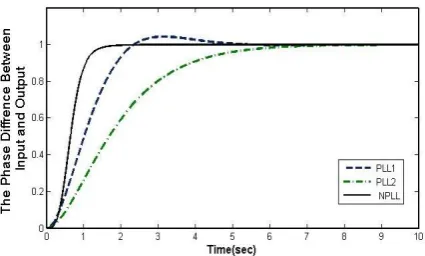
Fig. 9 The Phase step response of PLL₁,PLL₂ and NPLL

In Fig. 9 the step response of output phase of NPLL is closer to ideal step in comparison with PLL₁ and

2

PLL considerably; because of lesser settling time and rise time. Also, The NPLL hasn’t any considerable overshoot.

Table 1 shows the overshoot, rise time and settling time of the nonlinear PLL in comparison to two linear one. As it is shown the NPLL has better step response feature features rather than the two others.

Obviously if N has greater value, the approximation of f v( ) is more precise. The performance of NPLL for different value of N is shown by Table 2.

Fig. 10 shows that the step response for NPLL with the different number of coefficients. The phase step response is more close to ideal step while N=5 in comparison with other value of N which is confirmed by the result of the transient response. It must be mentioned that the overshoot is equal to zero for all NPLLs. In return for the accuracy of approximation of ( )f v , the running time of optimization program increases. This means that there is a trade off between the accuracy of approximation of f v( ) and optimization time.

Table 1 The performance measure of three PLLs

Overshoot (sec)

Rise time (sec)

Settling time (sec)

1

PLL 0 3.46 4.8

2

PLL 4.32% 2.35 4.8

NPLL 0 0.71 1.22

Table 2 The performance measure of three NPLLs

Running time (sec)

Rise time (sec)

Settling time (sec)

3

N = 315.67 0.76 1.31

4

N = 347.10 0.71 1.22

5

N = 367.29 0.64 1.10

Fig. 7 The sum of surfaces between ideal step and actual

response

Fig. 10 The Phase step response of NPLL for different number of coefficients N

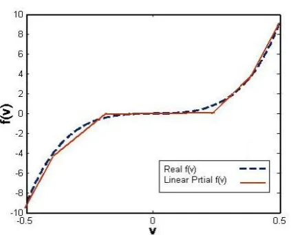
Fig. 11 The graph of f(v) and linear partial function for N=4

Table 3 The value of coefficients of ( )f v

a1 a3 a5 a7 a9

3

N = 0.33 45.0 94.1 - -

4

N = 0.17 54.4 54.7 78.0 -

5

N = 0.50 36.8 99.4 85.7 88.3

Table 3 shows the optimized coefficients of ( )f v for different value of N.

The nonlinear element of ( )f v could be approximated by linear partial function which is shown in Fig. 11. This graph function was simply implemented in CMOS technology [16-18].

6 Conclusions

This paper present a new structure for fast lock PLL based on embedding nonlinear element. In this method the Genetic Algorithm was used to find the best coefficients of nonlinear element. As it’s seen, the optimal nonlinear element increases the speed of PLL and simultaneously decreases overshoot .According to the results, using Genetic Algorithm for estimate the coefficients of nonlinear improve phase step response considerably.

References

[1] Razavi B., Design Of Analog CMOS Integrated, Circuits, Mc Grow Hill, 2001.

[2] Razavi B., Design of Monolithic Phase-Locked Loops and Clock Recovery Circuits-A Tutorial, Wiley-IEEE press,1993.

[3] Best, R. E., Phase-Lacked Loops: Design, Simulation and Applications, 5th edition, McGraw-Hill, New York, 1999.

[4] Razavi B., RF Microelectmnics, Prentice Hall, Upper Saddle River, NJ, 1998.

[5] Crawford J. A., Frequency Synthesizer Design Handbook, Artech House, Boston, MA, 1994. [6] Stephans D. R., Phase-Locked Loops for Wireless

Communications: Digital and Analog Implementations, 2nd edition Kluwer Academic, Norwell, MA, 2002.

[7] Egan F. W., Phase-Lock Basics, A Willy-Interscienc Publication,1998.

[8] Stensby J., “An Approximation of the Pull-Out Frequency Parameter in a Second-Order PLL,” Proceedings of the 38th Southeastern Symposium on System Theory Tennessee Technological University Cookeville, TN, USA, 2006.

[9] Shahruz S. M., “A Low-Noise and Fast-Locking Phase-Locked Loop,” Proceedings of the American Control Conference Denver, Colorado, 2003.

[10] Shahruz S. M., “Novel Phase-Locked Loops With Enhanced Locking Capabilities,” Proceedings of the American Control Conference Anchorage, AK, May 2002.

[11] Goldberg D. E., Genetic Algorithms in Search, Optimization and Machine Learning, Addison-Wesley, Reading, MA, 1989.

[12] Haupt. S. E, Haupt. R. L, Practical Genetic Algorithms, ISBN 0-471-45565-2, Wiley-Interscience, 2004.

[13] Kaya .N, Machining fixture locating and clamping position optimization using genetic algorithms, Department of Mechanical Engineering, Uludag University, Go¨ru¨kle, Bursa 16059, Available online 6 September 2005. [14] Chipperfield A. J., Fleming P. J. and Pohlheim

H., “A Genetic Algorithm Toolbox for MATLAB,” Proc. Int. Conf. Sys. Engineering, Coventry, UK, pp. 200-207, 1994.

[15] Sivanandam S. N., Deepa S.N., Introduction to Genetic Algorithms, Springer, 2008.

[16] Wilamowski B. M., Jaeger R. C. and Okyay kaynak M., “Neuro-fuzzy Architecture for CMOS implementation,” IEEE Trans. on Industrial Electronic, Vol. 46, Issue 6, pp. 1132-1136, Dec. 1999.

[17] Wang W. Z. and Jin D. M., “Neuro-fuzzy system with high-speed low-power analog blocks”, Elsevier Science J. Fuzzy Sets and System, No. 157, pp. 2974-2982, 2006.

[18] Wang W. Z., Jin D. M., “CMOS design of analog Neuro-fuzzy system with Improved circuits”, Proc. IEEE 7th International Conference on Solid-State and Integrated Circuits Technology, Vol. 2, pp. 1591-1594, Oct. 2004.

Mariam Zabihi received the B.Sc. degree in

2006 and the M.Sc. degree in 2009 in electronics engineering from Babol University of Technology, Babol, Iran. Her research interests are Signal Processing, Perturbation Methods, CMOS Analog Design.

Hossein Miar-Naimi was born in Chalous,

Iran, in 1972. received the B.Sc. from Sharif University of Technology in 1994 and M.Sc. from Tarbiat Modares University in 1996 and Ph.D. from Iran University of Science and Technology in 2002 all in Electrical Engineering respectively. Since 2003 He has been member of Electrical and Electronics Engineering Faculty of Babol University of Technology. His research interests are analog CMOS integrated circuit design, RF & Microwave microelectronics.