ψ
-Epistemic Models, Einsteinian Intuitions, and No-Gos
A Critical Study of Recent Developments on the Quantum State
Florian Boge
University of Cologne, Philosophy Department, University of D¨usseldorf, Philosophy Department/DCLPS
Abstract
Quantum mechanics notoriously faces the measurement problem, the problem that if read thoroughly, it implies the nonexistence of definite outcomes in measurement procedures. A plausible reaction to this and to related problems is to regard a system’s quantum state|ψimerely as an indication of our lack of knowledge about the system, i.e., to interpret itepistemically. However, there are radically different ways to spell out such an epistemic view of the quantum state. We here investigate recent developments in the branch that introduces hidden variablesλin addition to the quantum state
|ψiand has its roots in Einstein’s views. In particular, we confront purported achievements of a concrete model that has been considered to serve as evidence for an epistemic view of the envisioned kind, as well as specific no-go results and their import. It will be argued that while an epistemic account of the particular kind is not straightforwardly ruled out by the no-go results, they demonstrate that the evidential character of the model(s) discussed rests on a rather shaky foundation, and that they make some achievements widely recognized in the literature appear worthy of doubt.
Keywords: ontological models, PBR theorem,ψ-epistemic models, quantum mechanics
1. Introduction
Quantum mechanics (QM), construed broadly, is the scientific theory with the greatest practical impact and predictive success (cf. e.g. [2, p. 116] or [3, p. 893] for examples), and yet to date it is still faced with the infa-mous measurement problem (MP) – the problem that the unitary time evolution allows for and preserves superpo-sition states and thus provides no dynamics that lead to definite outcomes in measurement procedures – and with related issues, all ultimately rooted in quantum superpo-sition. Dirac [4, p. 7] and von Neumann [5, p. 217] his-torically attempted to solve the MP by adding the projec-tion postulate (PP) to the theory, which says that when observableAis measured on systemS in state|ψ(t)i, the state ofSundergoes a sudden change|ψi −→ Pˆa|ψi
kPˆa|ψik with
probability | ha|ψ(t)i |2. Here ˆP
a =|aiha|is the projection
operator onto the subspace spanned by |ai, so upon con-clusion of this process, the sate of the system is the (nor-malized) eigenstate |ai of A. In modern QM, this theme readily generalizes1 to L¨uders’ rule ρˆ −→ MˆmρˆMˆm†
Tr( ˆMmρˆMˆm†)
, where ˆρ = P
jλj|ψjihψj| is the system’s density matrix
1This is not to say that L¨uders’ rule is the general rule to
de-scribe state transformations; it rather “characterizes just one (albeit distinguished) form of state change that may occur in appropriately designed measurements of a given observable with a discrete spec-trum.” [6, p. 356]
that may represent amixed quantum state (in case there are two λj 6= λk which are both unequal to zero), and
where {Mˆ†
mMˆm}m∈I (I some indexing set) is some more
generalpositive operator valued measure (POVM). Many POVMs result from coarse-graining projector valued mea-sures (PVMs) [7, p. 3], and this “may or may not admit the kind of ignorance interpretation familiar from classi-cal physiclassi-cal experimentation.” [ibid.] The use of mixed states implies that nopure quantum state is assigned even beforehand, and (despite the non-uniqueness of decompo-sition of a mixed state) in particular cases this may be understood as an expression of the fact that the ‘true’ quantum state is simply unknown [cf. e.g. 8, p. 20]. To that extent generalized measurements may smell like epis-temic uncertainties being crucially involved in measure-ments in QM, and state changes being ‘merely informa-tional’ in some sense. It is not clear though that these considerations carry over to other types of measurement (or even to all generalized measurements), and on account of theeigenvalue-eigenstate link, i.e., that an observableA has value a on a system S iff the state of S is given by an eigenvector |ai of the operator ˆA representing A, the ‘sudden change’ mentioned above would clearly have to be interpreted differently.
ob-servation has a direct impact on physical reality (cf. [9]; [10]). Of course today we have a whole range of alter-native responses to the MP such as the may worlds in-terpretation, Bohmian mechanics, objective collapse the-ories... and what have you, all with their particular vices and virtues. There is, however, one particular response that sticks out in its ‘naturalness’, and it is certainly en-dorsed in some form or other by “[t]he philosopher in the street, who has not suffered a course in quantum mechan-ics” (Bell’s phrase [11]) and, we may add, by many a physicist in the lab who has not concerned himself with the foundations of QM. This response is to deprive even pure quantum states of their ontological significance, and to construe the theorynot as a description of the behavior of physical systems, but rather as a representation of the knowledge an actual or ideal observer or agent can have about these. On such a view, the need for an instanta-neous reduction of the state vector upon certain kinds of ‘measurement-like’ interactions is removed at once, and the ‘collapse’ appearing in the PP indeed comes out just a sort of informational update for the experimenter upon registration of a given result.
Interpretations of this general sort are typically called epistemic or ψ-epistemic. However, one can spell out an epistemic interpretation in multiple different ways, with strongly diverging underlying assumptions. Leifer for in-stance maintains that
it is important to distinguish two kinds of ψ-epistemic interpretation. The most popular type are those variously described as anti-realist, instrumentalist, or positivist. [...] The second type ofψ-epistemic interpretation are those that are realist, in the sense that they do posit some underlying ontology. They just deny that the wavefunction is part of that ontology. Instead, the wavefunction is to be understood as repre-senting our knowledge of the underlying reality, in the same way that a probability distribution on phase space represents our knowledge of the true phase space point occupied by a classical particle. [12, p. 72]
We are here concerned with epistemic interpretations of the second type in Leifer’s classification, the kind of in-terpretation of quantum states which is realist in a decisive sense and arguably strives for as much preservation of com-mon sense as possible. The decisive sense of realism here is at least a metaphysical or external one, meaning that “[t]he world is (largely) made up of objects that are mind-, language-, and theory-independent.” [13, p. 8] According to such a realism, there should be no doubt that every system always has a unique, definite state, a unique way of how it ‘actually is’, despite our ignorance of this ‘actual how’. This should also—a slightly stronger assumption— at least in principle enable us to give a unequivocal de-scription of that definite state. The ‘weirdness’ that QM
is notoriously associated with is just an expression of our inability to properlyaccess the true states of certain (typ-ically microscopic) systems, and hence it vanishes when properly construed in terms of incomplete knowledge.
2. Einstein’s Views and Hidden Variables
A central tenet underlying this type of epistemic inter-pretation is that QM is in fact an incomplete theory that will (hopefully) be replaced by a more complete and com-prehensive one in the future. This assumption surfaced early on when the peculiar features of QM became ap-parent, and its most prominent proponent was, of course, Einstein. This is most vividly reflected in his 1939 corre-spondence with Schr¨odinger, where he writes:
I am as convinced as ever that the wave rep-resentation of matter is an incomplete repre-sentation of the state of affairs, no matter how practically useful it has proved itself to be. The prettiest way to show this is by your example with the cat (radioactive decay with an explo-sion coupled to it.) At a fixed time parts of the ψ-function correspond to the cat being alive and other parts to the cat being pulverized. If one attempts to interpret theψ-function as a complete description of a state, independent of whether or not it is observed, then this means that at the time in question the cat is neither alive nor pulverized. But one or the other sit-uation would be realized by making an obser-vation.
If one rejects this interpretation then one must assume that the ψ-function does not express the real situation but rather that it expresses the contents of our knowledge of the situation. [14, p. 43]
Due to Einstein’s brave advocacy of these views, we here coin the kind of epistemic interpretation in question Einstein epistemic (EE). Due to Bohr’s immortal influ-ence on the other sort of epistemic interpretation (the first kind in Leifer’s classification), we will call it Bohr epis-temic(BE), in contrast. We emphasize that an EE account need not encompassall of Einstein’s views on the quan-tum state; we here merely use his core intuition, that “the ψ-function does not express the real situation but rather [...] the contents of our knowledge” to form a label.2
Ironically, youngHeisenbergalso spoke merely of a “de-struction of theknowledgeof a particle’s momentum by an apparatus determining its position” [15, p. 21; my empha-sis – FB], and while he himself went on to develop onto-logically more charged philosophical views of the quantum
2It will be interesting though to discuss at least to some extent
state, according to an EE view this is basicallyall there is to most if not all of QM’s weirdnesses.
But how does one spell out such an EE view in detail? Einstein’s writings are often associated with an ensemble interpretation of quantum states because of his continuing appeal to statistical ensembles, as witnessed, e.g., in his reply to criticisms in Schlipp’s volume on his life and work [cf. 16, p. 668], or in his 1936Physics and Reality, where he writes: “Theψ-function does not in any way describe a condition which could be that of a single system; it relates rather to many systems, to ‘an ensemble of systems’ in the sense of statistical mechanics.” [17, p. 375]
While there remains some controversy over what Ein-stein’s use of the word ‘ensemble’ actually entailed (cf. [18]; [19, p. 239 ff.]), a more explicit view of this kind was later defended and extended by Ballentine, who describes it in the following terms:
For example, the system may be a single elec-tron. Then the ensemble will be the concep-tual (infinite) set of all single electrons which have been subjected to some state preparation technique (to be specified for each state), gen-erally by interaction with a suitable appara-tus. Thus a momentum eigenstate (plane wave in configuration space) represents the ensem-ble whose members are single electrons each having the same momentum, but distributed uniformly over all positions. [20, p. 361]
The “state preparation technique” must in fact rather be viewed as anequivalence class thereof [cf. 7, p. 5], since it is possible to use either a calcite crystal or a grid po-larizer, say, to prepare a photon in a certain polarization state, and since different sets of preparation procedures can be used to prepare the same mixed state.
It may not be immediately obvious why this view of the quantum state should count as ‘epistemic’, but it is obvious from the above quote that at least Einstein was aiming for an epistemic interpretation. He may, in fact, have equally had in mind anideal orconceptual ensemble, as suggested in Ballentine’s quote, construed as a cognitive tool for de-termining probabilities of experimental outcomes. This is also the viewpoint of Harrigan and Spekkens [21, p. 150] who think that “the ensembles Einstein mentions are sim-ply a manner of grounding talk about the probabilities that characterize an observer’s knowledge [...]” and sim-ilarly of Bartlett et al. [22, p. 4] who believe that “the thesis that quantum states describe the statistical proper-ties of a virtual ensemble of systems [...] is equivalent to saying that it describes one’s limited information about a single system drawn from the ensemble.”
Butwhat exactly do these ensembles consist of? They cannot consist of conceptual electrons (say) in the sense of QM, because all QM assigns is the state vector which does not—andcannot—attribute definite values for all ob-servables at all times. So the conceptual ensembles must
consist of something else, something not exhaustively de-scribed by QM, but only by some set of additionalhidden variables.
Epistemic hidden variable approaches of course have a long history in QM as well, and they are the most explicit version of the general contention that QM is incomplete and that there are additional features in nature, more in line with the concepts of classical physics and everyday life thinking (cf. also [23, p. xvii ff.]). The assumption of hidden variables is also clearly presupposed by ensem-ble approaches such as Ballentine’s, as is evident from Whitaker’s analysis of them:
[I]f the wave-function of a free particle is an eigenfunction of momentum, all members of the ensemble will have the corresponding value of momentum, but in addition each has a pre-cise value of position, though these values will all be different. The values of position must be called hidden variables, because they are not related to the wave-function. [19, p. 210-211]
In fact, allmeaningful ensemble interpretations of QM have to assume hidden variables (as has also been cogently pointed out by Home and Whitaker [24, p. 263 ff.] and d’Espagnat [25, p. 297 ff.]). But there is also the rather trivial sense in which the term ‘ensemble’ plays a role in QM proper: since QM is concerned with probabilistic pre-dictions, the state function must always also be allowed to refer to an entire ensemble of equally prepared systems [cf. 23, p. 6]. If QM is considered to be complete however, thenψshould be taken to represent, at the same time, the state of anindividual system, which is decidedly not the case with probability distributions (or densities) used in classical statistical mechanics.
The traditional ensemble interpretations are conceptu-ally revisionary in this sense, in enforcing a break with the assumptions underlying orhtodox QM. But they are formally conservative: QMas it is may serve as a formal tool for devising statistical predictions; the possibility of a more complete physical theory endorsing hidden variables in a formally explicit sense is merely left open or hoped for.
There are, however, well known reasons why such for-mally conservative epistemic interpretations never really took off. Schr¨odinger [26, p. 156],3 for instance, started
developing counter-examples early on. One of his exam-ples was a harmonic oscillator with a given fixed value of total energy ((n+12)~ω for some fixedn, say). In the cor-responding quantum state of the system, an eigenstate of energy, there would be a large uncertainty as to the os-cillators position x. But according to an ensemble view, kinetic and potential energy, depending on velocity and position respectively, should be well defined at all times
3Cf. also [19, p. 214] for a more detailed analysis of Schr¨odinger’s
for each individual member of the ensemble (or rather: the physical objects referred to), whence there should be a clear cut-off value for the position. To see this, con-sider that the potential energy increases with position x
in the oscillator potential, and kinetic energy (increasing with velocity) cannot be negative (i.e., the oscillator does not ‘less than not move’), so that the limit (n+12)~ω in total energy implies a limit for possible positions. But QM of course predicts non-vanishing probabilities for positions beyond that limit.
Similar worries are raised by quantum tunneling. In α-decay, anα-particle has to tunnel through the Coulomb barrier of the nucleus in order to be emitted. This escape is impossible in a classical physical scenario, since the par-ticle would have to have greater potential than total en-ergy at some point, which again implies negative kinetic energies [cf. 19, pp. 214-215].
And finally, arguments that appeal to quantum inter-ference are typically invoked, since a simple statistical par-ticle interpretation does not predict the observed interfer-ence patterns in double slit experiments and the like. Only the incorporation of an active part of the diaphragm (and possible detectors behind both slits) may raise hopes for a suitable statistical analysis in terms of ensembles. Nothing of this sort is present in the formally conservative ensemble interpretations.
In summary, what these and many further examples show is “how far away from the basic [...] ensemble one has to go – [...] as Bohr would have stressed, one must include the measuring device as an active participator in the measurement, not just a recorder of a fixed value.” [19, p. 217] And the failure to do so may be seen as the major crux of the historical ensemble approaches.
3. Formal Revisions and Epistemic Models
Modern epistemic approaches in fact do use a revised formal inventory, including the possibility for an active part of the measuring device in producing the outcome statistics. From this, they can prima facie successfully reproduce many predictions peculiar to QM from merely epistemic restrictions – including examples of the infamous quantum interference phenomena.
A particularly influential formal framework that allows to formulate an epistemic view of quantum states in more detail, developed originally by Spekkens [27] and extended in joint work with N. Harrigan [21], and very much like (if not an instance of) the formalism used by Bell [28], is that of the so called ontological models (OMs).
3.1. The Ontological Models-Approach: General Outline
To define what an OM is, Harrigan and Spekkens pre-suppose anoperationalisticunderstanding of QM, which in their words means that “the primitives of description are simply preparation and measurement procedures – lists of instructions of what to do in the lab” [21, p. 128], and they
contend that the goal of this operational formulation is just to determine outcome probabilities for measurement procedures. In contrast, the primitives of description in an OM for this operational theory are the properties of microscopic systems (ibid.).
To match the operational reading with the quantum formalism, they associate apreparation procedure P with a density operator ˆρ (whereas Spekkens [27, p. 3], more accurately, associates an equivalence class of such with ˆ
ρ) and a measurement M with a POVM {Eˆj}j∈J. But
how, precisely, do we have to understand the ‘association’ ? Whatexactly does the quantum state represent about the system? The preparation procedure itself (or rather: its equivalence class)? That which results from it? A virtual ensemble in the sense of section 2? In contrast to Harrigan and Spekkens, Busch et al., for instance, write: “Any type of physical system is characterised by means of a collec-tion of preparacollec-tion procedures, the applicacollec-tion of which prepare the system in astateT. The set of states is taken to be convex, thus accounting for the fact that different preparation procedures can be combined to produce mix-tures of states.” [7, p. 5, emphasis in original] Here the state is namedin addition tothe collection of preparation procedures, as that which results from them. We will here hence make sense of the association as follows: The quan-tum state ˆρ of a given system is the state of the system according to its preparation, whence we may read the word ‘state’ in a decidedly non-ontological fashion: it does not represent how the system actuallyis, but rather what can besaid about it, in virtue of what wasdone to it. ˆρmay of course be a pure state and correspond to an eigenstate of some operator, whence the eigenvalue-eigenstate link is clearly severed in this approach.
Outcomes in projective measurements, however, can be identified with (pure) quantum states as well, whence quantum states should also be allowed to represent ‘states according to measurement’. Notably, this reading fits well with the general operationalism about QM, since the mea-surement is also an operation performed on the system and generally not so much different from the preparation procedure (think of a Stern-Gerlach measurement, where both preparation and measurement involve magnets and screens). Indeed, we thus preservehalf of the eigenvalue-eigenstate link, i.e. that when an observableAis measured to have valueaonS, the state ofSis given by|ai—though only in the operational reading of ‘state’.
In accord with our analysis, we will, in what follows, occasionally call ˆρ(orψ) theP/M-stateof a system. Given this understanding of quantum states, Born’s rule provides a probability PrρMˆ (k) = Tr( ˆEkρ) of obtaining valueˆ k in a
measurementprocedure of typeM given somepreparation procedure resulting in ˆρ, i.e., with the meanings of the indices of the probability function loosened.
specification of the properties of a system [...].” [21, p. 128] Talk of ‘ontic’ states, however, seems somewhat clumsy, whence we will prefer to speak of true states instead, i.e. states which are true of the systems under consideration, in a correspondence theoretic understanding of truth. This is what the OM approach (obviously) aims for.
In addition to the space of true states λ, two proba-bility densities are defined. The first one is termed epis-temic state, and is intended to reflect the knowledge a possible observer might have about the λ ∈ Λ. Hence it corresponds to a conditional probability p(λ|ρ) orˆ pρˆ(λ)
of obtaining a certain true state λ, conditional on having prepared P-state ˆρ. The second one, denoted byp(k|λ, M) orξMk (λ), is called anindicator-orresponse function,4and it is supposed to reflect uncertainties in a given measure-mentM leading to outcomek, conditional on the fact that stateλobtains on a system [27, 21].
To formally connect the probabilities occurring in the OM approach to the quantum probabilities, Harrigan and Spekkens [21, p. 128] require that an OM must respect the constraint
Z
dλ ξkM(λ)pρˆ(λ) = Tr( ˆEkρ),ˆ ∀ρ, Mˆ (1)
to be a model of QM. That is: adding up (integrating) all the probabilities of obtaining a given outcome k, given a certain measurementM and true stateλ, weighted by the probability that the state λeven occurs after having pre-pared ˆρ, must reproduce the quantum probabilities.5 This
fully defines what an ontological modelis,6the state space
Λ, the epistemic state and the response function, and the connection to QM given by formula (1). Hence ‘ontological model’ should be read here rather as atechnical term; not much ontology is actually conveyed. The OM approach provides a formal framework for analyzing different inter-pretations of QM, and sketches a road to modifications of QM’s formalism whichallowfor the specification of an on-tology in which the quantum state does not figure, or at least not fundamentally. It does not yet provide such an ontology.
Ipso facto, we are here dealing with an explicit hid-den variables-approach, the true statesλbeing the hidden variables. Generallyλneed not be interpreted as a hidden variable though, since it can be interpreted as the quantum state ψ itself—the OM-approach is formally neutral on this point. In fact, Harrigan and Spekkens [21, p. 129 ff.]
4Response functions in statistical mechanics need not be
normal-ized, and therefore need not be interpretable as probability densities in general. In the present context, we assume this to be the case though, in accord with the literature on the subject studied here.
5For the mathematically inclined, measure theoretic
generaliza-tions can be found in [12, p. 82].
6In [27], the possibility of including a transformation matrix
Γ(λ, λ0) in (1) is discussed, to the end of analyzing the notion of contextuality within the OM approach. We will not dedicate much attention the these here though, since contextuality is not a major subject of the paper.
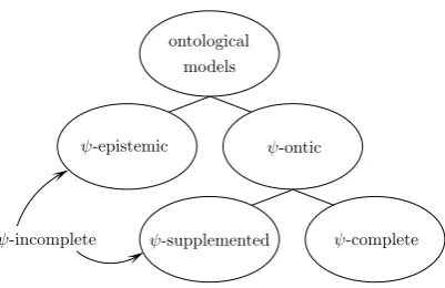
draw a multifold distinction between classes of OMs (cf. figure 1), with a dichotomy of ψ-onitc and ψ-epistemic models. Intuitively this means that the quantum state can either be construed as something that actually pertains to real, mind-independent systems, or instead something we ascribe to those systems only in virtue of our lack of knowl-edge about their true states. Within the first category they again distinguish ψ-supplemented from ψ-complete mod-els, where the former category simply consists of OMs in which the quantum state is something that pertains to reality, but still notall there is. Intuitively,Bohmian Me-chanics is an example of such a ‘model’, though it is not clear that it formally fits the approach [cf. 29]. The notion of ψ-complete models should now be self-explaining. For obvious reasons,ψ-epistemic andψ-supplemented models are jointly termedψ-incomplete.
To get a hold on the more precise definitions of the dif-ferent subclasses of models, it is sufficient to look into the definitions Harrigan and Spekkens provide for ψ-onticity and ψ-completeness, as the other concepts can be stated in terms of negations of these.
Definition(ψ-completeness). An ontological model is ψ-complete if the space of true states Λ is isomorphic to the projective Hilbert spaceP(H) (the space of rays of Hilbert space) and if every preparation procedure Pψ associated
in quantum theory with a given rayψis associated in the OM with a Dirac delta function centered at the true state λψ that is the value of ψ in the isomorphism, pψ(λ) =
δ(λ−λψ).7
Put frankly, this definition tells us that an OM is ψ-complete in case it reproduces QM tout court. The true states in Λ are bijectively mapped onto rays in Hilbert space, and the probability of a true state obtaining, given a preparation procedure associated with a ray inH, is such that it is 1 for the true state that is the value of the ray in the isomorphism, and zero for all other true states. The quantum statistics is reproduced in a trivial fashion.
As we saw, the notion ofψ-onticity is supposed to allow for supplementation ofψ by elements of the model which do not simply mirror elements of QM, whence a ψ-ontic model is defined as follows.
Definition(ψ-onticity). An ontological model isψ-ontic if for any pair of preparation procedures, Pψ and Pφ,
as-sociated with distinct quantum states ψ and φ, we have pψ(λ)pφ(λ) = 0 for allλ.8
In other words, the supports of two epistemic states that are conditional on two different procedures for prepar-ing distinct P-states should not overlap (on sets of non-zero measure). Now ψ-ontic models which do not satisfy
7Cf. [21, p. 131]. We have slightly altered the wording in the
definition, as Harrigan and Spekkens callλψ andψisomorphic, but
it is meaningless to talk ofelements of spaces as ‘isomorphic’. The appeal to projective space Hilbert space here is due to the invariance of quantum states under multiplication by a global phase.
ψ-epistemic ψ-ontic
ψ-supplemented ψ-complete ψ-incomplete
ontological
models
Figure 1: Classification of OMs according to the status of the quantum state.
the first definition are calledψ-supplemented, non-ψ-ontic models are called ψ-epistemic. The decisive criterion for a model to be ψ-epistemic is hence that there be an over-lap in (the supports of) the epistemic states associated with distinct quantum states. The intuition being that, if it may happen that λis really the case in two instances, and we have prepared for ψ in the one and for φ in the other, then ψ andφ themselves do not reflect something pertaining to the system. Given that the probability dis-tributionspρˆ(λ) were supposed to represent “what can be
known and inferred by observers” [21, p. 129], this can be translated more crisply into the statement that one can-not know/infer for sure that a given λ is not sometimes the case when one prepares for ψ, and sometimes when one prepares for φ.
Note that sometimes modifications to the definition of ψ-epistemicity are discussed [e.g. 30] such that an overlap is only required for non-orthogonal states, since two or-thogonal states|φi,|ψimay be construed as indicative of mutually exclusive preparation procedures that could ar-guably result in mutually exclusive sets of true states, or even that all non-orthogonal states should be associated with overlaps [e.g. 31]. We here however stick to the def-inition given above, and the negation of ψ-onticity here merely implies the existence of two such distinct (possi-bly non-orthogonal) states that have distributions associ-ated to them with overlapping supports. This is a com-paratively weak requirement, and refinements in terms of distance measures between the epistemic states have also been proposed (see e.g. [32, p. 477]; [33, p. 2]).
Again, we find justification for associating this kind of epistemic interpretation with Einstein, since the idea of demonstrating the incompleteness of QM in virtue of the existence of twoψ functions that correspond to the same real physical state of an object at the same time was also explicitly advocated by him:9 “[...] co¨ordination of several
ψ functions with the same physical condition of [some] system [...] shows [...] that the function cannot be inter-preted as a (complete) description of a physical condition
9This is also a key reason why Harrigan and Spekkens [21] devote
a large part of their paper to Einstein’s views of the quantum state.
of a unit system.” [17, p. 376] We repeat, however, that the OM approach in general merely constitutes a formal framework for analyzing different interpretations of QM or of the quantum state. Here we are only interested in the approach to the extent that it can accommodate the intuitions underlying an EE view, i.e.: we are here only concerned with ψ-epistemic models, and we take them to be a suitable implementation of an EE view.
3.2. Interlude: The Philosophical Issues at Stake
What is at stake in the present discussion of the quan-tum state? In fact, there is a whole range of topics that could be picked out, but we will focus on three concerns and how they relate to the debate.
The search for ‘completeness’ is our first concern, and it raises some first worries as regard the definitions at hand. Recall thatλwas supposed to correspond to a “complete specification of the properties of a system[...].” But on a broad reading of ‘property’ this seems rather impossible. For suppose that we have prepared forψ in the one case and φin the other, and that in both cases λis supposed to occur. Then we can say that there is a (complex) rela-tional property of being-in-a-Pψ-situation in the first case,
and a relational property of being-in-a-Pφ-situation in the
second, and hence,λcannot strictly specifyall properties. Bell, whose work has certainly served as a paradigm for the OM approach (as noted above), more cautiously talked about a “more complete specification”, for which it is “a matter of indifference [...] whether λ denotes a single variable or a set, or even a set of functions, and whether the variables are discrete or continuous.” [28, p. 15; my emphasis – FB] Clearly Harrigan and Spekkens must have in mind a particular set of physical or natu-ral properties; kinematical quantities comparable to those arising from the phase space formalism in classical mechan-ics, i.e. all (and only) those properties that can be defined in terms of (generalized) positions and momenta. Ruetsche [34, p. 31] in fact makes a point in our favor, in iden-tifying generalized coordinates and momenta as paradig-matic examples of magnitudes she calls “fundamental in the physicist’s sense,” meaning that it is usually assumed that the value of every other magnitude pertaining to a system can be determined by assigning values to these on the system. The ‘completeness’ sought for by Harrigan and Spekkens must consist in seeking such fundamental-in-the-physicist’s-sense quantities. Quantum mechanically the closest analogy is the complete set of comeasurable ob-servables. But since these of necessity only include a sub-set of all conceivable observables, the contention (again) is that there must be other, hitherto undiscovered magni-tudesbeyond QM’s observables that are more in line with the classical description.
system in an ontologically privileged way? As regards use-fulness, QM proper arguably has quite an edge in the light of all its predictive and technological successes—despiteits lack of definite descriptions similar to the those occurring in classical theories. So seeking completeness in more than a theory-internal sense first of all requires a sensible crite-rion for naturalness of properties.
Besides the completeness-issues, a second point to won-der is what concept(s) of probability are involved in ψ-epistemic models. This is a point which Harrigan and Spekkens refrain from elucidating, as they “do not feel that the distinction [between different concepts of probability – FB] is significant in this context [...].” [21, p. 150] This distinction may not be as insignificant as they apparently believe though, since (famously) there is a whole host of radically differing views of probability, and opting for one particular view always comes with rather deep ontological and epistemological implications. Possibly the broadest dichotomy one can draw is that between epistemic and objective probabilities [cf. e.g. 35, p. 2], and on this coarse level the classification of the epistemic state seems pretty clear. But as regards the response function, matters are more subtle. Harrigan and Spekkens here have it that “the model may be such that the ontic state λdetermines only the probability p(k|λ, M) of different outcomes k for the measurement M.” [21, p. 128; my emphasis – FB] And this smells like the response function involving objective probability. But in fact they also claim that “p(λ|P)and p(k|λ, M) specify what can be known and inferred by ob-servers” [21, p. 129; my emphasis – FB], whichprima fa-cie conflicts the previous quote. But remember that their claim merely was that an (epistemic) OM leaves it open whether (“may be such that”)λdetermines only outcome probabilities for valueskin measurementM. And if there is indeed a random response of the measurement device to the true states fed in, then it is, of course, also the case that only a probability for a given outcome can be known or inferred by an observer.
For the purposes of an epistemic model, one might still be inclined to hope for an interpretation of the re-sponse function according to which randomized rere-sponses “could occur because of our failure to take into account the precise ontological configurations of either [preparation or measurement]” [36, p. 4], or simply reflect an “unknown disturbance” [37, p. 10; my emphasis – FB] of the sys-tem caused by the measurement—much like Heisenberg’s elimination of knowledge due to the measurement process. However, taking both probabilities to be epistemic in this sense could, firstly, be fleshed out to yield a kind of mi-crodeterminism, meaning that on a sufficiently fine-grained scale of observation (accessible only to Laplacian demons, as it were), no probabilities would be needed. This would take the debate to a whole other level though, since cur-rently the central question is one of microdefiniteness(the existence of additional true states which explain the mea-surement statistics), not determinism. And secondly, we saw that a failure to take the role of the measurement
de-vice into account was the main reason for the failure of the historical (ensemble) approaches, so regarding the re-sponse function as merely reflecting epistemic uncertain-ties may not be good advice after all, or at least raises further concerns.
Leifer [12, p. 70], moreover, notes that “calling a proba-bility density ‘epistemic’ [...] presupposes a broadly Bayes-ian interpretation of probability theory in which probabil-ities represent an agent’s knowledge, information, or be-liefs.” But ‘broadly Bayesian’ may still be too broad in this context, since there is also thequantum Bayesian ap-proach, which explicitly endorses subjective Bayesianism and refrains from entertaining (formally explicit) hidden variables. Consider Williamson’s [38, p. iii] characteri-zation of the distinction between subjective and objec-tive Bayesianism: “Subjecobjec-tive Bayesians hold that it is largely (though not entirely) up to the agent as to which degrees of belief to adopt. Objective Bayesians, on the other hand, maintain that appropriate degrees of belief are largely (though not entirely) determined by the agent’s evidence.” Moreover, Williamson characterizes objective Bayesianism as a normative theory, i.e., a theory which claims that “[t]he strengths of an agent’s beliefs should behave like probabilities[...].” [38, p. 1; my emphasis – FB]
Prima facie ψ-epistemic models, in which the epis-temic state quantifies what can be known and inferred by observes, are best construed as embracing an objec-tive Bayesian reading of probabilities. But upon closer in-spection, they also appear compatible equally with what Williamson [38, p. 15] refers to asempirically based subjec-tive Bayesianism. All forms of Bayesianism, Williamson (ibid.) tells us, hold a Probability norm, meaning that “one’s degrees of belief at a particular time must be prob-abilities if they are to be considered rational.” Empirically based subjective Bayesians add a Calibration norm, i.e. that “one’s degrees of belief [...] should also be calibrated with known frequencies.” (ibid.) Because the epistemic state is supposed to reflect what can be known and in-ferred by an observer (agent) – on the basis of evidence about preparation methods, and the presumed range of true states which can result from each preparation – we can see that the attribution of probabilities must be on the ba-sis of known frequencies, and the Calibration norm should clearly hold forψ-epistemic models. Objective Bayesians additionally assume anEquivocation norm, meaning that “one’s degrees of belief at a particular time are rational if and only if they are probabilities, calibrated with physi-cal probability and otherwiseequivocatebetween the basic possibilities.” [38, p. 16; my emphasis – FB] It is not clear that an epistemic OM must embrace this norm as well, but we will investigate a particular model below which clearly does.
realist. In fact, all the issues at hand, the status of the epis-temic probabilities, the search for completeness, and the status of the quantum state, all boil down to questions of the precise kind of realism endorsed.
It has been criticized though, in particular by Norsen [39], that in certain applications in the context of QM (the violations of Bell-type inequalities) the discussion is blurred by the use of the word ‘realism’, because “it is almost never clear what exactly a given user means by the term [...] and [...] none of [the] possibly-meant senses of ‘realism’ turn out to have the kind of relevance that the users seem to think they have.” [39, pp. 311-312] Whether Norsen’s assessment is correct is open to debate. But we concede that there is a crucial terminological problem that we should try to fix.
First of all we note that the ψ-epistemic OMs need not be consideredna¨ıvely realist in the sense appealed to by Norsen [39, p. 316], namely in the sense that “when-ever an experimental physicist performs a ‘measurement’ of some property of some physical system [...] the outcome of that measurement is simply a passive revealing of some pre-existing intrinsic property of the object.” (emphasis omitted) This, Norsen thinks, is the physics-appropriate generalization of “the view that all features of a perceptual experience have their origin in some identical correspond-ing feature of the perceived object.” (p. 315)
Classicalphysics is typically taken to entertain exactly that sort of na¨ıve realism, as it seems to endorse that measurements can at least in principle be as subtle and non-invasive as desired (think again of Heisenberg’s “de-struction of knowledge”, which he apparently considered as a philosophical revelation). Similarly, the ensemble ap-proaches discussed in section 2 may be classified as na¨ıvely realist, but, again, ψ-epistemic OMs neednot be viewed as na¨ıvely realist in Norsen’s sense, since both prepara-tion and measurement are infected with uncertainties, so that pre-existing intrinsic properties of systems are not just revealed passively10– at least as long as the response
function is interpreted objectively.
More illuminatingly, it appears that the project of find-ing ψ-epistemic models for QM must embrace a form of scientific realism (i.e., that (i) mature and well confirmed theories are capable of being true, and (ii) the concepts of these very theories typically do refer to entities in the external world, inalldomains, including unobservable mi-crostates [cf. 40, p. xvii]), since scientific methods are em-ployed to seek out (refer to) the true states of investigated systems. But since QM is interpreted operationally, this realism can only (or at least: mostly) be endorsed here w.r.t.classical physical concepts and theories.11 The fact
that inψ-epistemic models, the aim is to reduce quantum
10By judging thusly, we are in fact disagreeing with Norsen, who
thinks that this na¨ıve realism is the idea of a non-contextual hidden variable model. But the disagreement may be based on the under-standing of ‘context’.
11Note that, if scientific realism was applied here to the concepts
of a hitherto undiscovered physical theoryT, this would not be more
probabilities to classically interpretable ones, and quan-tum states to definite states that provide a (more) com-plete specification of reality should suffice as evidence for this claim. Grossly speaking, we can hence classify EE views asselectively scientific realist.
Peters [41, p. 377] describes selective scientific realism as the view “that not all the propositions of an empirically successful theory should be regarded as (approximately) true but only those elements that are essential for its suc-cess”, but he also notes that “[i]t is [...] not obvious how a term like ‘essential’ is to be understood.” If we apply this reading of ‘selective’ to the present case, what would be such essential elements? We may take it that the possibil-ity of a rather gapless (formal)picture of reality is consid-ered somewhat essential to scientific theories by advocates of an EE view, since the supplementation of additional variables to the formal inventory (instead of an analysis of the formal elements already present in QM) would oth-erwise be a moot point. And indeed, Spekkens generally characterizes OMs as “an attempt to offer an explanation of the success of an operational theory by assuming that there exist physical systems that are the subject of the experiment.” [27, p. 2]
We can see that rather deep philosophical issues are at stake here, and the OM approach provides not only a technically useful basis for the general discussion of in-terpretations of QM, but also for the assessment of these very issues in the context of QM. But to assess whether epistemic models formulated in the approach can ascer-tain the completability of QM, the suitability of objective (or empirically based subjective) Bayesianism for the in-terpretation of probabilities in QM, and a selectively sci-entific realist attitude for the general context, we must ask: (i) Are there any models which fit the definitions from section 3.1, and (ii) to what extent can these repro-duce the empirical predictions of QM? Indeed, Harrigan and Spekkens provide examples of models for each of their categories, but we here turn to a model that Spekkens has devised in 2007 instead, and which, we here take it, has so far brought about the greatest apparent successes in pro-viding evidence for an EE view. We will here grossly focus on this model to evaluate (ii).
3.3. Spekkens’ Toy Model
What we here call a ‘toy model’ was originally devel-oped by Spekkens [37] under the name “toy theory”, but it can be fit into the OM approach, as shown in [12, p. 84] and below. The toy model is only concerned with analoga of qubit systems (i.e. systems with only two relevant states in QM), but can be expanded to include systems of mul-tiple, coupled qubits. The analogues of qubits in the toy
than a merehope forscientific realism. Moreover,T would still have to imply classical physical theories in suitable limits, and sinceT
is decidedlynot QM, we can take it that an EE view seeks out a
model are called elementary systems (cf. [37, p. 3]). For these elementary systems, Spekkens postulates four pos-sible true states, simply denoted by {1,2,3,4}. There is a foundational principle at the heart of this model, called thekowledge balance principle:
Knowledge Balance Principle (KB). If one has max-imal knowledge, then for every system, at every time, the amount of knowledge one possesses about the [true – FB] state of the system at that time must equal the amount of knowledge one lacks. [37, p. 3]
This, of course, immediately raises the question of how to measure knowledge. To provide a measure, Spekkens first defines what he calls canonical sets (cf. ibid.):
Definition (Canonical set). A canonical set is a set of yes-no questions that is sufficient to fully specify the true state, and that has a minimal number of elements.
To understand this notion, consider that if one only knows that the state of the system under investigation is in the set{1,2,3,4}and one wants to find out in which of the states it actually is, one could ask “Is it in state 1?”, “Is it in state 2?”, and so forth. Or one could be smart instead, and just ask, say, “Is the system’s state in the set
{1,2}?”, and “Is the system’s state in the set{2,3}?” Two nos will give assurance that it is in state 4, two yeses that it is in 2, and one yes and one no that it is either in 1 or 3, depending on the order. Now the amount of knowledge one has is defined within the toy model as “the maximum number of questions for which the answer is known, in a variation over all canonical sets of questions.” (ibid.).
(KB) then dictates that one can always only know half the answers in such a set, and this is somewhat reminis-cent of an epistemic reading of the uncertainty relations. Applied to physical systems such as spinful particles, we can understand it such that, “if we know thex-coordinate [of spin – FB] with certainty then we cannot know any-thing about the y-coordinate.” [12, p. 73] Put frankly, this means that the epistemic states (for simple systems) within this model must be distributions which assign prob-ability 1/2 to two states, and probprob-ability 0 to two others. That is, we can always know that the state is in a subset like {1,2}, but nothing more.
To connect these principles to QM, consider (as does Spekkens) the following six quantum states, which are the only P/M-states of the model:
|0i, |1i,
|+i=√1
2(|0i+|1i), |−i= 1
√
2(|0i − |1i),
|+ii=√1
2(|0i+i|1i), |−ii= 1
√
2(|0i −i|1i),
withh0|1i= 0. Accordingly our epistemic states will be of the formp(λ|x), λ∈ {1, . . .4}, x∈ {0,1,+,−,+i,−i}.
Since we are only concerned with a discrete set of pos-sible true states, the probability distributions can be
rep-resented by n-tuples. This also means that condition (1) which connects the QM probabilities with the probabilities in the OM must be changed to a sum:
Tr( ˆEkρ) =ˆ
X
λ∈Λ
pρˆ(λ)ξMk (λ). (2)
Spekkens also introduces a convenient notation for the epistemic states, which we will equally make use of in what follows. We hence make the following identifications:
p0= (12,12,0,0)!1∨2, p1= (0,0,12,12)!3∨4,
p+= (12,0,12,0)!1∨3, p−= (0,12,0, 1
2)!2∨4,
p+i = (0,12,12,0)!2∨3, p−i = (12,0,0,12)!1∨4,
Curvy arrows are used to denote correspondence between different notations, and the disjunctions should be read ‘merely symbolic’ at this point (we will spend a few thoughts on connections to logic below). We have, e.g., p0(1) =
p0(2) = 12 andp0(3) =p0(4) = 0.
The response functions turn out deterministic here; for instance,
Pr|+/0i−(+) =| h+|0i |2= 1/2 !
=X
λ∈Λ
p0(λ)ξ++/−(λ),
where ‘+/−’ refers to the measurement associated with outcomes + and−. But this means that ξ+/+ −(λ) has to give 1 for the first of theλs, and cannot also give 1 for the second one. Equally,
X
λ∈Λ
p1(λ)ξ+/+−(λ) !
=| h+|1i |2= 1/2,
X
λ∈Λ
p+(λ)ξ+/+−(λ) !
=| h+|+i |2= 1,
X
λ∈Λ
p−(λ)ξ+/+−(λ) !
=| h+|−i |2= 0,
and so forth. All in all, we get ξ++/−(λ) = (1,0,1,0), so that theξfor outcome + mirrors thepwhich is conditional on +, but with 1s instead of 12s. All theξs can be worked out to look this way.12
So ξ actually does not do any work here at all and could be omitted altogether. Models of this kind have been coined maximally ψ-epistemic (cf. [30, p. 2]; [42, p. 4]), and the toy model is such a maximally epistemic model.
With this simple setup, Spekkens is prima facie able to reproduce a bunch of quantum phenomena. To this end he assumes measurements to be “reproducible in the sense that if repeated upon the same system, they yield the same
12Note that it is not a contradiction that the entries inξsum up
outcome.” [37, p. 9; emphasis in original] In other words: they are like the projective measurements of QM. But as noted before, due to (KB) measurements cannot reveal the true state λ, but can only change what one knows about the system. To elaborate, first note that a state of total ignorance, where one only knows λ ∈ {1,2,3,4}, should be described by an epistemic statep(λ) = 1/4,∀λ∈Λ, or 1∨2∨3∨4 [37, p. 4].13
Upon measurement 1∨2∨3∨4 will now be changed into a state where one knows one of the (symbolic) disjunc-tions 1∨2,3∨4,1∨3. . .This is represented in the model as the measurement ‘inducing a partition’, say{1,2,3,4}−−→M {{1,2},{3,4}}. This amounts to aprobability update, rem-iniscent, of course, of Bayesian condtionalization [cf. 38, p. 75 ff.]. Let us say that some experimenter has no prior knowledge about the true state of a system, and hence no preference in belief as to which state an inves-tigated system is in. Then her epistemic state should be p = (14,14,14,14). Upon measuring the value + (say), she will instantaneously think that the system must be in one of the states 1 and 3, but she can still give no preference to any of the two. Thus her knowledge about the system has to be represented as p+= (12,0,12,0). This is the
pic-ture provided by the formal setup of the model of what happens in a measurement, and it seems to explain the presence of the projection postulate in orthodox QM.
It is important to note that (KB) is restricted to the knowledge about a systemat a given time. This is so be-cause given that one knows 1∨2, a measurement which partitions {{1,3},{2,4}} will lead to definite knowledge of the state of the system prior to the measurement; in case one measures 1∨3 the state must have been 1, in case of 2∨4 it must have been 2. The fact that one still lacks complete knowledge about the system’s state after the measurement is accounted for by an “unknown dis-turbance” of the state, caused by the measurement [37, p. 10].
The first achievement of this model now is that these measurements can be demonstrated to exhibit non-commutativity, just as quantum measurements do. Con-sider two measurements A and B inducing partitions
{{1,2},{3,4}} and {{1,3},{2,4}} respectively, and per-formed on a system in state 1∨2. Performing the A-measurement first will keep the system in 1∨2 and the B-measurement will then yield 1∨3 and 2∨4 with equal fre-quencies. Performing them the other way around, the B-measurement will first update the epistemic state to either 1∨3 or 2∨4; but now theA-measurement will yield 1∨2 and 3∨4 with equal frequency. This should be compared, say, to the non-commutativity of spin measurements along orthogonal axes in a Stern-Gerlach experiment.
13Since nothing at all is known in states like 1∨2∨3∨4, this
can also be construed to mirror completely mixed states that can be decomposed into multiple convex combinations [cf. 37, p. 5]. We here also see that the modelequivocatesbetween basic possibilities, which substantiates our previous claim that it is objectively Bayesian.
|0i
|1i |+i
|−i
|−ii |+ii
1∨2
3∨4 1∨3
2∨4
1∨4 2∨3
(a) (b)
ˆ
U=√1 2
1 i i 1
P=
1 2 3 4 2 3 1 4
Figure 2: (a) is a regular Bloch sphere for the qubit states, (b) is an analogous diagram for the epistemic states (cf. [37] for a similar illustration). Two of these can be combined by opera-tions +1, . . . ,+4to yield one of the respective other states, just
as two quantum states can be superposed to yield a third one. In (a), transformations are represented by unitary operators (which can be mapped onto rotations), in (b) permutations are used instead.
Another achievement is the (partial) reproduction of quantum superposition. This is accomplished by defin-ing different rules for combindefin-ing the epistemic states. For instance, one could combine two states such as 1∨2 and 3∨4 by taking the true state of lowest index and combining them into a new state, i.e. 1∨3. This may be symbolized by writing (1∨2) +1(3∨4) = 1∨3. Equally, we could
take the true states of highest index to obtain 2∨4, which may be written as (1∨2) +2(3∨4) = 2∨4. Taking one of
higher and one of lower index from both epistemic states respectively will yield two further possibilities (+3and +4;
cf. [37, p. 6]). With these four combination rules, the in-terrelations of all six quantum sates considered above can be mirrored, which is best illustrated in terms of Bloch spheres (or Bloch sphere-like diagrams), as in figure 2.
There are, however, a few subtleties involved in this analogy which lead into a (first) kind of trouble. Combin-ing, say, (2∨3) +4(1∨4) = 2∨4 in the toy model should,
according to the Bloch sphere-image, be analogous to su-perposing|+iiand|−iito get |−iin QM, i.e. developing
|−i = h+i|−i |+ii+h−i|−i |−ii = 1+i2 |+ii+ 1−2i|−ii. A complication is now raised, however, by the fact that combination rules +3 and +4 have a particular ordering
sensitivity, as e.g. (1∨4) +4(2∨3) = 1∨36= (2∨3) +4
(1∨4). One can model this situation by a superposition
1 √
2(|+ii −i|−ii) with relative phase, which is equal to
e−iπ
4 |−i, because
e−iπ4 = cos
−π
4
+isin−π
4
=
= cosπ 4
−isinπ 4
=√1
2(1−i),
so that
e−iπ4 |−i=√1
2(1−i)|−i= 1
√
2(|+ii −i|−ii).
includes a relative phase of 3π
2 (sincee i3π
2 =−i) between
the two states superposed. In fact, the four combination rules above can all be understood in terms of quantum superpositions with a relative phase, and Spekkens [37, p. 7] makes the following identifications:
+1!+ei·0, +2!+eiπ,
+3!+ei π
2, +4!+ei 3π
2 .
These identifications reveal the subtleties mentioned above and show that the analogy between combinations of epis-temic states and quantum superpositions is not—and can-not be made—perfect. In the given choice one obtains (1∨3) +3(2∨4) = 2∨3 and (1∨3) +4(2∨4) = 1∨4,
but √1
2(|+i+e iπ
2|−i) =ei π
4 |−iiand √1
2(|+i+e i3π
2 |−i) =
e−iπ4 |+ii, which, given the identifications between
combi-nation rules and epistemic- and quantum states, should be exactly the other way around. Exchanging identifications in the latter case will always only shift the problem [cf. 37, p. 7]. According to Spekkens (ibid.), “[t]his curious failure of the analogy shows that an elementary system in the toy theory is not simply a constrained version of a qubit.”
So the toy model fails to correctly reproduce the QM toolkit from epistemic restrictions in this instance, and is bound to do so. But this need not be a strong objection to the general enterprise yet, because (a) we are here dealing with a limited toy model only, and (b) it should not be required that any successful alternative to QM must mir-ror the quantumformalismisomorphically; a successful re-placement of, or alternative to QM should only be required to preserve QM’s successfulpredictions. If we construe the model, however, as a first approach toreducing the exact rules of QM to incomplete knowledge (thereby serving as evidence for an EE view), then it must still appear as a drawback that the model fails to do so.
Be that as it may, further interesting phenomena can (apparently) be reproduced within the toy model in virtue ofstate transformationsbeing represented in the model as permutationsof true states in the epistemic state, or equiv-alently, as resamplings of the epistemic state (cf. figure 2). In the Bayesian paradigm, this amounts to a change in an observer’s knowledge, the point being that the true state of a system does not have to change, even if the epistemic state of an observer does. One can of course find out some new piece of information, regardless of whether the sys-tem this information is about remains entirely unchanged. Intuitively we can access the formal analogy to unitary transformations in the Bloch representation, as the latter correspond to rotations (up to an overall phase) of point-ers inside the sphere, and permutations will also appear as rotations by angles ofnπ
2(n∈Z) in the toy sphere (cf.
figure 2 (b)).
But what is striking about permutations as state trans-formations is that they seem to make the reproduction of quantum interference examples possible. To elaborate,
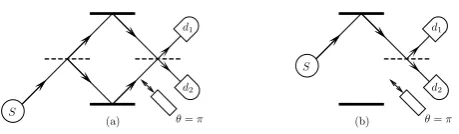
θ=π d1
d2
S
BS1 BS2
Figure 3:Mach-Zehnder interferometer with an optional phase.
consider the following setup14 based on a Mach-Zehnder interferometer (figure 3), where one photon at a time en-ters the setup, emitted from a source (S) towards a 50/50 beam splitter (BS1), so that there will be a 50/50 chance
for each photon of passing throughBS1 or being reflected
at a right angle.
Neglecting polarization etc., we can model this as a simple spatial qubit of a ‘moving up state’|%i=. 1
0
and a ‘moving down state’ |&i=. 0
1
(‘=’ implies a choice of. representation). Now take a photon prepared as|%ibyS. BS1 will change the state into a superposition of moving
up and moving down, represented by
ˆ
UH|%i=
1
√
2(|%i+|&i) =:|ψi, (3)
ˆ
UH =. √12 11 −11
theHadamard gate.
Imagine now that behind each beam of photons ema-nating from BS1 there are mirrors (the thick black lines
in figure 3), aligned such that both trajectories are de-flected towards each other again. We can represent the transformation effected by the mirrors by the ˆσx
Pauli-matrix, which will only exchange the flying up- and down-components of|ψiand hence essentially leave it untouched, as
0 1 1 0
1
√
2
1 1
= √1
2
1 1
.
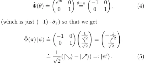
We can also insert a phase shifter in the lower branch, say, but after the mirrors, so that it will only affect the flying-up part of the spatial sflying-uperposition state. If we choose θ=πas our phase, we will obtain a transformation which can be represented by the matrix
ˆ Φ(θ)=.
eiθ 0
0 1
θ=π
=
−1 0 0 1
, (4)
(which is just (−1)·ˆσz) so that we get
ˆ
Φ(π)|ψi=.
−1 0 0 1
√1
2 1 √ 2
!
= −
1 √ 2 1 √ 2
!
. = √1
2(|&i − |%i) =:|ψ
0i. (5)
But in case we insert a second beam splitter (BS2 in the
14Note that no analogous discussion of such an example is provided
figure) at the point where the two trajectories cross, |ψ0i
will change as
ˆ UH|ψ0i
. = √1
2
1 1 1 −1
−√1
2 1 √ 2
!
=
0
−1
.
=− |&i. (6)
So our simple qubit model predicts that we will always find a down moving photon in this setup, which has only picked up an unobservable phase of π(eiπ=−1).
Computing the probabilities for detecting an up- or downward traveling photon at the end of this setup gives, of course, | − h%|&i |2 = 0 and | − h&|&i |2 = 1. The
relative phase between two kets is entirely responsible for the precise resulting behavior atBS2;15without the phase
we would instead have
ˆ UH|ψi
. =√1
2
1 1 1 −1
√1
2 1 √ 2
!
=
1 0
.
=|%i, (7)
i.e. only photons movingup at the end of the setup. To check the predictions of this model one can use de-tectors (d1andd2in figure 3) which give off a perceivable
signal (a click if you will) upon incidence of a photon. With the phase shifter in place this (ideally) means only detections in d2, and without the phase shifter (ideally)
only in d1, and experiments of this kind have of course
been successfully performed [43].16
Since the setup contains only one photon at a time, it seems surprising that it should matter to a photon travel-ing along the upper path whether there is a phase shifter in the lower one. But still, an analogous example can be constructed in the toy model by appeal to permutations instead of unitary matrices. The simplest type of permu-tation is a swap of two elements in an ordered sequence, and we will describe all permutations occurring in the ex-ample in terms of such swaps here. Thus, let (jk) repre-sent the swap of elementsjandkin some orderedn-tuple (n≥j, n≥k). Then in the toy model we start out with 1∨2 !p% as the epistemic state corresponding to the
preparation of|%i(=|0i). The first beam splitter is rep-resented by a permutation (23), which results in 1∨3 (i.e. 3 will now be assigned the probability previously assigned to 2, which is 1
2). The mirrors can be represented by (13),
yielding 3∨1 = 1∨3, so that not much happens here, just as in the QM treatment. In case the phase shifter is in, this can be modeled as a permutation corresponding to
15Note that we have assumed both arms of the interferometer to
be of equal length, so that none of the two states can pick up a phase due to spatial delay.
16In fact, varying the phase somewhat more than justθ∈ {0, π},
one can appeal to probabilities of detection in eitherd1ord2, where
Prψθ
x (d1) = | h%|ψθi |2 = cos2(θ2) for |ψθi := 12
(1−eiθ)|&i+
(1 +eiθ)|%i, as results from the setup with a general phase shift.
One can equally use a difference in path length, as mentioned in footnote 15, and this is what was done in [43], to confirm that the number of counts would conform to the predicted cos2-regularity.
two successive swaps (12)(34) which then yield 2∨4. And the second beam splitter will again correspond to (23), so that the final state is 3∨4. But this distribution is the one corresponding to the quantum sate|1i=|&i so that the quantum predictions are indeed preserved. Equally, if the phase shifter is not inserted, this means that the permutation (12)(34) is left out, whence 1∨3 will just be transformed into 1∨2 at the second beam splitter, and we obtain the state that we started off with, again just as in QM.17
Thus the toy model can indeed reproduce interference examples with the aid of resamplings of probability distri-butions. And resamplings can result in the toy-analogue of superpositions just as unitary transformations can result in quantum superpositions. We have here considered only a limited example with a certain fixed phase, but a mathe-matical generalization of Spekkens’ work exists [44] which can handle arbitrary phase arguments in terms of proba-bility vectors and transformation matrices. This achieve-ment has lead several authors to conclude that “a whole host of Mach-Zehnder interferometry experiments can be qualitatively reproduced by the theory[...].” [12, p. 79]18
“But hold on!”, you may interject, “How can a lack of knowledge account for the fact that what I do in the lower arm of the interferometer will influenceall photons in the setup, even if they take the upper route?” And as well you should. We have here rather ‘blindly’ applied the for-mal tools of the toy model, which then appeared to nicely mirror some features of QM. But that permutations can be made to look like rotations on the Bloch sphere, and that these rotations in turn are homomorphic to unitary operations is a long shot from accepting that resamplings of a probability distribution (construed as a formal repre-sentation of a change in knowledge) can account for what goes on in a Mach-Zehnder interferometer. How is it that our knowledgeshould be affected by the putting in of the phase shifter?
For all we know, many of the true states of systems in the setup—those representing something moving through the upper route—should not be affected at all, whence, a fortiori, neither should our knowledge of them. Build-ing the example bottom-up, we would certainly not have guessed that putting in a phase shifter must result in in-terference, in case only one photon enters the setup. It is only our background knowledge of QM and the confirming experiments that allows us to concoct the toy model in the appropriate way, and it leaves us without any explanation as towhy our knowledge should change in this way. To be fair, we should here take into account that Spekkens aims to “identify phenomena that are characteristic of states of
17All of these swaps can be implemented in the form of
transforma-tion matrices, as indicted in footnote 6. If one uses columns instead of rows to represent the epistemic states, (23) on 1∨2, say, takes on the simple form
1 0 0 0 0 0 1 0 0 1 0 0 0 0 0 1
! 1/2
1/2 0 0
!
=
1/2 0 1/2
0
!
.
incomplete knowledge regardless of what this knowledge is about.” [37, p. 2] A possible move at this point is thus to counter that we are informed by our experience with Mach-Zehnder interferometers, and that we should, in ac-cord with the Calibration norm, adapt our epistemic states to the known frequencies in experiments with or without phase shifter.
Still, there is some tension with the general philosoph-ical stance of an EE view, as we have identified it in previ-ous sections. A key motivation for an EE view is a certain preservation of common sense to secure a thorough basis for metaphysical realism. In particular, the introduction of true statesλwas identified to ensure microdefiniteness, and as such it raises hopes for finding a more complete physical theory that makes it possible (in principle) to give an account of how the world is (beyond the QM descrip-tion). Thus if the project is to serve its principal goal, it should at leastallowfor an ontology of the true states that provides an explanation of the situation in question.
Hence: What do 1,2,3,4 represent, and how are they affected by the setup in such a way that the kind of prob-ability update exemplified above is indicated? In fact, Spekkens and others seem to feel this need for explanation as well whence thereis a kind of (ex post) explanation in the literature (cf. [47]; [45]; [12]). But we will only be able to suitably assess its plausibility after a discussion of two no-go theorems below.
We should now also look at combined states of two (or more) simple systems in the model. Loosely follow-ing [37, p. 11 ff.], we can represent the simultaneous oc-curence of two true states i, j ∈ {1, . . . ,4} on two dis-tinct systems a, b respectively by a (symbolic) conjunc-tioni(a)∧j(b). Of course having such an epistemic state is prohibited by (KB) since it would correspond to com-plete knowledge of the true states of both systems. But combinations of epistemic states, i.e. states of the form [j(a)∨k(a)]∧[`(b)∨m(b)], with j, k, `, m ∈ Λ, and j 6= k, `6=m, are possible. These mimic simpleproduct states of QM, such as |ψ(a)i |φ(b)i.
A second possibility are states of the form [j(a)∧k(b)]∨
[`(a)∧m(b)]∨[n(a)∧o(b)]∨[p(a)∧q(b)] withj6=`6=n6= p, k6=m6=o6=q. I.e.: it could be known, say, that both systems are in the same state, but not inwhich state. Or it could be known that both are in different states, related by a certain specified permutation (transformation), but not which is in which. States of this form are supposed to mimic entangled states, and prima facie they do capture the essence of such states quite well.
To see this, take two systems which have been prepared in an entangled state, say |πi= √1
2(|0,0i+|1,1i). Then
this state implies that there is a probability of 1/2 for each (sub)system to exhibit either of the two measurable val-ues (0,1), but both systems are bound to exhibit the same value if the same observable is measured on them. Now consider a situation in which the two systems are sepa-rated spatially and two agents, A and B or ‘Alice’ and
‘Bob’, as they are usually called, perform measurements on them. Then at the very moment Alice measures ‘1’, she will know that Bob will measure ‘1’ as well, in case he measures the same observable. Phrased in terms of knowl-edge this is not so much of a surprise, but if we would en-dorse the orthodox interpretation instead, with its sudden change in the system’s actual state due to the measure-ment, then Alice would be capable of ‘steering’19 Bob’s
system into some definite state, by choosing a certain kind of measurement to perform on her system—and suppos-edlyinstantaneously so atarbitrarily large distances.
From the point of view of the toy model this surprising consequence dissolves. Alice’s state prior to measurement should be represented as [1(a)∧1(b)]∨[2(a)∧2(b)]∨[3(a)∧
3(b)]∨[4(a)∧4(b)], since she knows that both systems are in the same state, even though she cannot know in which one. Accordingly, the measurement must result in some-thing like [1(a)∨2(a)]∧[1(b)∨2(b)], say. Treating the connectives in these symbolic formulae as actual conjunc-tions and disjuncconjunc-tions as in propositional logic for the mo-ment, the latter statement straightforwardly follows from [1(a)∧1(b)]∨[2(a)∧2(b)] by case distinction and adding disjuncts. But the other, more important direction is not straightforwardly valid, since [1(a)∨2(a)]∧[1(b)∨2(b)] is also true if [1(a)∧2(b)] holds, and taking into account that states pertaining to the same system mutually exclude each other,20 [1(a)∧1(b)]∨[2(a)∧2(b)] would actually be false. With the epistemic state as given above however (the fourfold disjunction) and mutual state exclusion on the same system, Alice can draw the appropriate conclu-sion.
Let us say that Alice chooses to measure{{1,3},{2,4}}
on her system and finds 1∨3. Then she will come to know thatbothsystems must be in either ofthosetwo true states (1 or 3). If she decides to measure{{1,2},{3,4}}instead and finds 1∨2, then she comes to know that both sys-tems must be in one of these states. So in fact performing both measurements in a row and obtaining these respec-tive results Alice can come to the conclusion that both herand Bob’s system must have been in state 1 all along. So she instantaneously obtains information about the dis-tant system. But since the act of measurement effects and unknown disturbance, the states of both systems may now (after both measurements) be different; the state of her system (a) could have changed to 2, in virtue of the disturbance effected by the second measurement. And as-suming Bob performs the same protocol, he need not even obtain outcome 1∨2 in the second measurement, since his system’s state could have been changed to 3 in the first measurement and then 3∨4 would result in the second case. All that Alice can come to know is hence that dur-ing the first measurement both systems were in state 1;
19This is the much-used term introduced by Schr¨odinger [48,
p. 556].
20It would hence be more appropriate to use exclusive disjunction
˙