www.wind-energ-sci.net/2/189/2017/ doi:10.5194/wes-2-189-2017
© Author(s) 2017. CC Attribution 3.0 License.
Statistical characterization of roughness uncertainty and
impact on wind resource estimation
Mark Kelly and Hans E. Jørgensen
Wind Energy Division/Meteorology Section, Risø Lab./Campus, Danish Technical University, Roskilde 4000, Denmark
Correspondence to:Mark Kelly ([email protected])
Received: 10 October 2016 – Discussion started: 1 November 2016 Revised: 20 January 2017 – Accepted: 21 February 2017 – Published: 25 April 2017
Abstract. In this work we relate uncertainty in background roughness length (z0) to uncertainty in wind speeds, where the latter are predicted at a wind farm location based on wind statistics observed at a different site. Sensitivity of predicted winds to roughness is derived analytically for the industry-standard European Wind Atlas method, which is based on the geostrophic drag law. We statistically consider roughness and its corresponding uncertainty, in terms of bothz0derived from measured wind speeds as well as that chosen in practice by wind engineers. We show the combined effect of roughness uncertainty arising from differing wind-observation and turbine-prediction sites; this is done for the case of roughness bias as well as for the general case. For estimation of uncertainty in annual energy production (AEP), we also develop a generalized analytical turbine power curve, from which we derive a relation between mean wind speed and AEP. Following our developments, we provide guidance on approximate roughness uncertainty magnitudes to be expected in industry practice, and we also find that sites with larger background roughness incur relatively larger uncertainties.
1 Introduction
Microscale flow models have been employed for decades in wind energy assessment to estimate resources at one loca-tion based on wind measurements at a different site (Troen and Petersen, 1989). Furthermore, it has become increasingly popular in the past decade to use mesoscale model output to drive microscale models for the same purpose (e.g., Bad-ger et al., 2014). Such flow modeling relies on characteri-zation of the surface, including terrain elevation and surface roughness. As input to atmospheric flow models, both terrain elevation and roughness have uncertainties associated with their assignment. In practice, terrain elevation uncertainty tends to be dominated by the resolution of elevation maps (e.g., Sørensen et al., 2012)1. In contrast, there are a number
1Currently (2016), microscale models typically have
computa-tional resolutions finer than elevation maps; commonly available el-evation maps in most of the world today have typical resolutions of 1x∼10–90 m, whereas quasi-linear (e.g., WAsP) and Reynolds-averaged Navier–Stokes (RANS) models employed for wind are
of significant uncertainties associated with roughness, which do not (necessarily) depend on resolution; these include de-termination of roughness lengthz0 from measurements and assignment ofz0 in industrial practice (based on land use, terrain type, and/or experience, for example). Overall, un-certainty related to roughness tends to be dominant over elevation-related uncertainty, particularly in wind-energy ap-plications. In this work we develop a practical treatment of the effect of roughness uncertainty upon wind resource esti-mation, providing a formulation for estimation of roughness-induced uncertainty in annual energy production.
First we review the definition of roughness length, in-troducing and demonstrating the statistical character ofz0, i.e., distributions ofz0 from measurements and the behav-ior of such; we statistically connect this to a practical
certainty metric. Then we present the theoretical frame-work that is used for wind resource estimation based on the geostrophic drag law (as used in the European Wind Atlas (EWA) methodology; Troen and Petersen, 1989) and includ-ing its relation to roughness. In Sect. 3 we introduce uncer-tainty; this includes basic characterization of the uncertain-ties inherent in (1) the roughness definition and observed distributions of z0 (Sect. 3.1.1) and (2) the variations inz0 prescribed in the wind energy industry (Sect. 3.1.2). We con-tinue by showing how uncertainty in the background rough-ness can be translated into uncertainty in predicted wind distributions, within the European Wind Atlas framework (Sect. 3.2.1); here we provide derivations of the sensitivity of predicted winds to input roughnesses at observation and prediction sites. Consequently, we examine the effect of user-assigned biases in roughness assignment and more generally the combined effect of (independent) roughness uncertain-ties on predicted wind speeds. For practical use we also de-velop an analytical relation between rated power, mean wind speed (Weibull-Aparameter), and AEP; this is accomplished via convolution of a generalized analytical power-curve form and Weibull wind distribution. Thus, we translatez0 uncer-tainty into unceruncer-tainty of annual energy production (AEP).
Though there are different methods possible for determin-ing or calculatdetermin-ing roughness length, we concentrate here on the propagation of uncertainty in background roughness to predicted wind speeds and annual energy production. More details about and issues arising from alternate methods of roughness length calculation are beyond the scope of this ar-ticle and are the basis of concurrent work to be included in a separate paper(s).
Lastly, we discuss approximate roughness uncertainty magnitudes expected in practice and the consequences of them. This also includes, for example, the result that sites with larger background roughness tend to give larger relative uncertainty (i.e., %) in predicted wind speeds and significant uncertainty in AEP. We also discuss implications for the use of mesoscale simulation data for driving microscale models, i.e., generalization of wind statistics.
2 Basis and framework
Physically, this work simply considers the use of wind mea-surements (statistics) at some height above ground level at one location in order to predict wind statistics at another lo-cation and height. Starting with ideal (uniform flat) terrain, this prediction can be broken into components, commonly labeled within the wind resource assessment community as vertical and horizontal extrapolation. Subsequently, the the-oretical foundation of this work involves the two basic com-ponents related to the physics modeled by such extrapola-tions: these are the wind profile for vertical extrapolation and the geostrophic drag law (GDL) for relating the wind statis-tics at different sites; they are covered in Sect. 2.1 and 2.2,
respectively. The vertical wind profile form (of which the simplest is the logarithmic law) requires a surface rough-ness length, and the GDL also requires a characteristic (back-ground) roughness length. Because we wish to relate uncer-tainty in roughness to unceruncer-tainty in wind energy estimates, i.e., finding the uncertainty in accounting for the effect of the surface, we first begin by examining roughness length, both in theory (i.e., definition) and in practice (e.g., its statistical character).
2.1 Roughness length: theory and practice
The concept of roughness length began with characteriza-tion of the velocity profile in ideal engineering flows (e.g., pipes), where roughness has a direct physical interpretation (Nikuradse, 1933; Tripp, 1936); it was further adopted to describe the wind profile in the atmospheric surface layer (ASL), whereby it has an implicit (and not directly physi-cal) definition (Monin and Yaglom, 1971). The basic role of roughness length and its definition, can be seen through the ideal expression for the mean wind profileU(z) over a homo-geneous flat surface in neutral conditions (without thermal stability effects):
U(z)=u∗ κ ln
z
z0
. (1)
In Eq. (1) z0 is the roughness length and z the height above (distance normal to) the surface, expressed in the same units;κ is the von Kármán constant, generally accepted to be 0.4 (Högstrom, 1996). The friction velocityu∗is defined byu2∗≡ −hu0w0i, i.e., as mean momentum transport towards
the surface through turbulent stream-wise (u0) and vertical or surface-normal (w0) velocity fluctuations. The roughness
z0 can also be seen as an integration constant since Eq. (1) results from integrating dU/dz=u∗/(κz); the latter is typ-ically derived via dimensional analysis, through the Buck-ingham Pi theorem (e.g., Stull, 1988; Wyngaard, 2010). The logarithmic wind profile (Eq. 1) depends upon a number of assumptions:u∗is effectively constant from the surface up to heightz(i.e., du2∗/dzσu2/`ABLWyngaard, 2010), the sur-face is flat and uniform, there is horizontal homogeneity (no variations parallel to the surface), there is no height depen-dence in the forcing of the flow, and there are (no effects due to) temperature variations, i.e., the only variables determin-ing dU/dzareu∗andz.
2.1.1 Calculation of roughness length from wind measurements
From Eq. (1) one can see that forUmeasured at two heights {z1, z2}, the roughness can be calculated by
ln(z0)=
U(z2) lnz1−U(z1) lnz2 U(z2)−U(z1)
. (2)
energy, Eq. (2) does not involve approximations and directly follows from the definition of roughness. One can also use friction velocity measured in the surface layer and wind speed from one (or more) height(s) to derive roughness (e.g.,
z0=zexp[−κU(z)/u∗]from Eq. 1), but doing so requires sonic anemometers, which are not yet commonly used in the wind energy industry. Thus, we use Eq. (2) for the observed roughness data analyzed and shown in this paper, and leave alternatez0estimation methods for concurrent work and dis-semination that focuses solely upon roughness. This choice is further supported by the focus of the present article – we are concerned here with the impact of roughness length on wind energy estimates – and because we develop and use an uncertainty-estimation framework that is generally applica-ble toz0, regardless of whetherz0is derived from Eq. (2) or viaU/u∗.
2.1.2 Roughness as a statistic
Even in seemingly ideal conditions – such as measuring wind profiles in the surface layer at a site where the ter-rain is flat and appears uniform, with non-neutral cases ex-cluded – in practice one still observes a broad range of roughnesses. This is demonstrated in Fig. 1, which shows the roughness length calculated from 10 and 40 m measure-ments at the Danish National Wind Turbine Test Station at Høvsøre for upwind directions corresponding to flat and ho-mogeneous surfaces (east of the meteorological measure-ment mast). Here we have filtered out non-neutral conditions by keeping only cases unaffected by thermodynamic stabil-ity by usingz/|L|<0.001, i.e., for Obukhov lengthsLmuch greater than the heights of measurement.
Figure 1 starkly demonstrates that even at a homogeneous, well-studied, and presumably simple site, roughness length has a distribution of significant width. Note that we plot the distribution of roughness length in logarithmic space; this is done because it is ln(z0) that directly affects the wind profile, as in Eq. (1). This also highlights the breadth of the distribution (several orders of magnitude) and that we must subsequently approach roughness uncertainty in a mul-tiplicative(dimensionless) way and not in an additive way. We also remind that the roughness lengths generally used in wind flow modeling and resource assessment actually corre-spond to some geometricmean, which should be based on thez0distribution (alternately one can express wind profiles in terms of the distributionP(lnz0) and corresponding arith-metic mean; cf., Kelly and Gryning, 2010); unfortunatelyz0 is not (yet) defined explicitly as such in typical wind engi-neering practice. Thus, in this paper we focus on roughness uncertainty within the “implied mean-roughness” framework implicit in standard wind engineering.
In addition to the relatively wide distribution apparent for roughnesses obtained from 30 min averages shown in Fig. 1 (and slightly wider for 10 min averages, not shown), one can also see some local – and nonideal – details. One sees the
minor effects of a barn and a small building located roughly 800 m upwind at∼80 and∼110◦, respectively, as well as
the larger effect of the seasonally varying marsh–fjord coast-line 800–900 m to the southeast (∼130–135◦). Such rough-ness changes tend to violate the assumptions behind the log-arithmic profile over a range of observation heights falling within the nonequilibrium internal boundary layer (IBL) transition region (Sempreviva et al., 1990; Bou-Zeid et al., 2004; Calaf et al., 2014)2. The more drastic semi-coastal roughness change contaminates the shear measured between 10 and 40 m enough to give the larger apparentz0shown in Fig. 1b asφ→135◦and the subsequently wider distribution
P(z0) shown in Fig. 1a for the 120◦sector.
Because neutral conditions tend to be encountered most often (stability distributions have their peak aroundL−1=0; see Kelly and Gryning, 2010), the distribution of shear expo-nentP(α) can also be related in terms of an effective rough-ness length without filtering stability to exclude non-neutral conditions (Kelly et al., 2014a). Thus, the wind profile can indeed give information about the surface, though the shear at higherz includes the effect of increasingly more terrain further upwind (potentially including hills as well as rough-nesses)3.
Avoiding substantial changes in surface characteristics and/or land use, this can be useful towards the aim of gauging backgroundz0.
One can also calculate a more local roughness length via Eq. (1) using measurements of U and u∗ within the surface layer (filtering out non-neutral conditions via mea-sured heat fluxes), but doing so requires sonic anemome-ters, which are not (yet) commonly used in the wind indus-try. For example, usingU andu∗measured atz=10 m for the case above givesP(z0, φ) that is insensitive to the inho-mogeneities described above, i.e., it does not jump asφ in-creases above∼130◦. Although the resultantz0(U/u∗) tends to better conform to the assumptions behind surface-layer theory and Eq. (1), it is consequently limited to ASL heights – which in stable conditions (e.g., nighttime, winter) only ex-tend to∼10–20 m. Furthermore, thez0derived fromU/u∗in the ASL is local, only pertaining to the nearest several hun-dred meters, perhaps less in stable conditions. However, the widths ofP(lnz0) derived fromU/u∗(not shown) are on par with those obtained fromUat two heights and displayed in Fig. 1.
Thus, in the present article concerned about uncertainty, we do not address the implications of surface-layer theory
2The IBL develops downwind from a roughness change with
ex-pansion slope (z:x) of roughly 1 : 100, and the top of the associated transition region expands at a variable rate of 1 to∼12–15. For the example noted here, this corresponds to the flow measured by anemometers at both 10 and 40 m being affected.
3The increasing area of surface affecting winds at increasing
Figure 1.(a)Distribution ofz0for homogeneous land sectors (30◦wide) east of Høvsøre.(b)Joint distribution ofz0and wind direction φ; darker represents most common values, and white is no occurrence. Calculation follows Eq. (2), withz1=10 andz2=40 m, and it is limited to neutral conditions (|L|−1<0.001 m−1).(c)Visual map east of site (red pointer; southern border of homogeneous zone at∼130◦ denoted by yellow line).
nor its conditional violation, but rather focus on the effect of roughness uncertainty – as it would be measured (or as-signed) in industrial practice – upon resource assessment, particularly through horizontal extrapolation from an obser-vation mast to a separate turbine location(s).
2.2 Geostrophic drag law: European Wind Atlas method
The geostrophic drag law (GDL) allows wind statistics ob-served at one site to be applied at potential wind farm sites nearby that may have different surface characteris-tics (i.e., roughness and terrain elevation); it is the ba-sis of the EWA method (Troen and Petersen, 1989) used widely for wind resource estimation. The GDL arises from matching the dimensionless surface-layer profile of mean wind in neutral conditions (i.e., the log law divided by u∗) to dimensionless solutions of the mean horizontal equa-tions of motion away from the surface, as affected by the Coriolis force (Ellison, 1956; Krishna, 1980; Walmsley, 1992). The mean atmospheric boundary layer (ABL) flow is driven by a large-scale mean pressure gradient ∇P, also expressible as the geostrophic windG≡ − ˆk×∇P /(fρ)= {−∂P /∂y, ∂P /∂x}/(fρ), where kˆ is the vertical unit vec-tor andf is the latitude-dependent Coriolis parameter; the pressure gradient force is balanced (vectorially) by the Cori-olis force and momentum transfer to the surface. Thus, the GDL essentially relates the large-scale forcing (expressible as the geostrophic wind above the ABL) to the surface-layer momentum flux (friction velocity), depending on the surface roughness.
The geostrophic drag law can be simply expressed in scalar form as
G=u∗ κ
s
ln u∗/f
z0
−A0 2
+B02, (3)
whereA0andB0are empirical constants (taken by the EWA to be 1.8 and 4.5). Thus, for two sites that can be assumed to have the same large-scale forcing (distribution ofG), then the wind statistics at one site can be translated to wind statis-tics at the other. From the wind profile relation (Eq. 1) one can obtainu∗from measuredUover one roughnessz0,1, and subsequentlyGfrom Eq. (3); then at the prediction site one can solve Eq. (3) to getu∗at a potential turbine site and sub-sequently findUthere over a roughnessz0,2. Below, we will show the impact of roughness uncertainty upon wind speed and AEP estimates via Eqs. (1) and (3).
3 Uncertainty
3.1 Roughness and uncertainty components
In general, uncertainty can be classified into two types (Ki-ureghian and Ditlevsen, 2009): aleatoric uncertainty, and
epistemicuncertainty.
First, aleatoric (sometimes called statistical or random) uncertainty is the variability in a quantity that arises from randomness inherent in the process(es) that impact said quan-tity.Epistemicor systematic uncertainty arises due to lack of knowledge about a quantity (imperfect understanding of it in the real world).
of the observed distribution ofz0shown in Sect. 2.1.2. This tends to be due to variability in the system being described; the system in this case is the atmospheric surface layer and the surface nearby the measurement point that influences the flow. However, there is also an epistemic component con-tained within the distributions P(z0) shown in Fig. 1; it is due to effects that were neglected in the derivation of the the-ory used, namely the logarithmic law (Eq. 1). Physically, this includes inhomogeneities in the surface upwind and depen-dence of surface characteristics upon wind speed (i.e., water or flexible vegetation; see Monin and Yaglom, 1971); within the context of the turbulent surface layer as described by tur-bulence theory, it tends to be manifested via turbulent trans-port (Kelly et al., 2014a; Sogachev and Kelly, 2016).
When performing resource assessment, in practice wind engineers characterize the surface via roughness length (as well as terrain elevation, which we do not treat in this pa-per). Roughness characterization can occur via assignment ofz0values chosen by the wind engineer or through rough-ness values (or land-use types) inherited from maps acquired from a third party. Typically, the former has dominated the wind industry, though the latter is becoming more common; land-use types and classes are contained in some geograph-ical data products, but these have not yet been shown to be consistently or universally translatable to roughness lengths for different parts of the world (see, e.g., Marticorena et al., 2006; Torbick et al., 2006). Either way, epistemic uncertainty arises due to our ignorance of the appropriate representative roughness length4and is introduced when characterizing the surface via a single roughness; this uncertainty exists regard-less of whether the characteristicz0is chosen by an algorithm assigning values to a map based on look-up tables for various land classifications or by a wind engineer who has visited the (potential) site.
The epistemic components associated with the theory used to convert; wind observations into observedz0tend to man-ifest via turbulent transport and subsequently behave ran-domly, arising to a good degree of variability of the surface itself (hence being debatably aleatoric). These are in contrast to the uncertainty arising from selection ofz0by engineers or the uncertainty inherent in (usage of) a relatively small num-ber of widely used sources for roughness maps, which can contain significant bias and are not (directly) related to mea-surement. Thus, here we group the former, observationally related uncertainty together with the aleatoric uncertainty, and then separately consider the epistemic uncertainty im-plicit in assignment of roughness values by wind engineers in practice.
4As shown in the section above, the representative roughness length should be based on ageometric mean, due the ln(z0) behavior exhibited by the surface-layer wind profile in neutral conditions.
3.1.1 Uncertainty in observation-basedz0
For the observation-based roughness lengths displayed in Sect. 2.1.2 (Fig. 1), the distributions are best described (and thus plotted) asP(lnz0), again consistent with both the ln(z0) behavior expected within the wind profile and with the geo-metric (multiplicative) averaging needed to obtain a charac-teristic mean roughness. The width of the ln(z0) distributions shown in Fig. 1 gives indication of the variability in lnz0over many 30 min (or 10 min) periods. In particular theP(lnz0) for 30◦-wide directional sectors can be considered, that is
P(lnz0|ϕ), since sectors of this width are commonly used in resource assessment. The homogeneous 60 and 90◦ sec-tors at Høvsøre (Fig. 1) have similar shapes, and both exhibit half-peak widths of roughly one-half order of magnitude (a factor of∼3); i.e., for a given sector’s background roughness
z0, the width of the distribution can be seen as that defined roughly betweenz0/3 and 3z0.
However, the uncertainty in determining a representative roughness length – via the appropriate (geometric) mean – is not the same as the width of the ln(z0) distribution. Rather, the uncertainty in the mean roughness is the width of the dis-tribution of expected means calculated for a given site and sector. For this purpose we use a basic “bootstrap” resam-pling method (Varian, 2005; Wu, 1986): simply resamresam-pling randomly from the diagnosed (30 min) roughness lengths, we synthesize a distribution of 105 values of geometric-mean roughness (hz0ig) per sector. This results in a log-normal distribution of meanz0(Gaussian distribution of lnz0); this distributionP(exp [hlnz0i]) is centered around a value equal to the geometric mean that had been found for each sector by operating directly on the wind data. The width of each (sector-wise) distribution of mean roughnesses from resam-pling depends on the number of resampled points used to cre-ate each mean in the synthesized distribution. For a number equivalent to 1 year’s worth of data (based on the sector-wise frequency of occurrence), the mean distributions are in fact much narrower than the distributions shown in Fig. 1. The bootstrapped mean-roughness distribution is almost perfectly fit by a log-normal form; the half widthwhz0iRSfor this form can be simply expressed non-dimensionally (i.e., effectively normalized by the expected mean) via the standard deviation of mean lnz0from resampling (σhlnz0iRS) as
whz0iRS
hhz0iRSig
=expnσhln[z0/hz0ig]iRS
o
=expσhlnz0iRS −1. (4)
For the Høvsøre homogeneous land sectors treated here and the bootstrapped means, each calculated from 1 year’s worth of resampled data, thewhz0iRSof the sector-wise distri-butions of these means are about 5 % of the expected mean roughness length (specifically, 5.4, 4.1, and 5.3 % of the re-spectiveh
Table 1.Means (geometric and arithmetic) and corresponding deviations inz0, surveyed from two groups of wind resource experts for the two terrain types shown in Fig. 2. For conventional (linear) standard deviationσz0, number in parenthesis isσz0/hz0i, given for comparison
with the logarithmic standard deviation (exp{σln
z0/hz0ig
}).
Geom. mean,hz0ig Arith. mean,hz0i exp
n
σln
z0/hz0ig o
Standard Deviation,σz0
Group Grass Forest Grass Forest Grass Forest Grass Forest n
Vindkraft-net 4.0 cm 0.87 m 5.6 cm 1.6 m 124 % 162 % 6.4 cm (115 %) 2.5 m (158 %) 28 DTU Wind 4.2 cm 0.82 m 5.5 cm 1.0 m 112 % 113 % 4.7 cm (86 %) 0.57 m (57 %) 19 Combined 4.1 cm 0.85 m 5.6 cm 1.3 m 117 % 141 % 5.7 cm (103 %) 2.0 m (146 %) 47
is about 5 %. For longer data sets, the uncertainty decreases; for example, randomly drawing from the entire 10-year set leads to half widths of 1–2 %.
One should be reminded that there are other methods to calculatez0, such as using the surface-layer friction velocity u∗and wind speed at one (or more) measurement height(s) via Eq. (1), which may result in different values of estimated mean and/or characteristic roughness length. For example, repeating the analysis above using Eq. (1) with U andu∗
measured at 10 m height, we again obtain well-behaved dis-tributions of bootstrapped mean roughness whose half widths are about 5 %; one might take this as the implied uncertainty. However, the mean values (for a given sector) can actually differ between the two methods by an amount that can greatly exceed 5 % (in these Høvsøre land sectors they can differ by a factor of ∼3!). This difference is related to the flow physics at increasing distances from the mast (the momen-tum flux footprint), the details of which are beyond the scope of this paper; we defer further discussion of such differences to Sect. 4.
3.1.2 Uncertainty and ensembles of user input
Even for an ideal homogeneous landscape, the wind industry, which is a collection of wind engineers and companies, will as a group assign different roughnesses to characterize the surface (whether actively or inherited via acquired maps). This results in a distribution of z0 assigned to predict the wind for any given site, and in effect to an (epistemic) uncer-tainty, and subsequently industry-wide variation in predicted AEP, even at the most simple sites.
We provide a simple practical example of gauging such epistemic uncertainty based on a systematic exercise: we asked separate groups of wind resource assessment experts to individually evaluate the surface roughness length for two commonly encountered land surface types. The groups of participants in this exercise were polled at meetings of the Danish Wind Power Network “Vindkraft-Net” (Kelly and Jørgensen, 2014) and of the Meteorology section of the De-partment of Wind Energy (Risø lab/campus) in the Danish Technical University; their backgrounds and foci range from
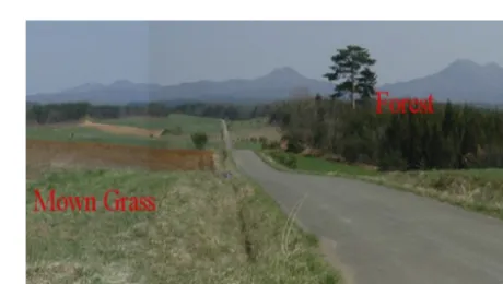
Figure 2.Image of the two areas (grassy and forested) used in roughness survey exercise.
wind engineering and commercial site assessment to research boundary-layer meteorology and wind resource calculation.
The participants were shown a picture containing both a grassy area and a forested area (the latter specified as having a mean tree height of 15 m) and were asked to givez0 for each of these two areas; the picture is replicated in Fig. 2. The raw results of the roughness survey, which consisted of 19 and 28 participants are shown in Table 1.
Note that Table 1 includes not only a geometrically defined
meanhz0ig≡
n
Q
i
(z0)i1/n=exp
n P
i
ln(z0)i/n
and
associ-ated dimensionless standard deviation exp{σln[z0/hz0ig]}that
are consistent with the logarithmic definition of roughness, but also the commonly used arithmetic mean and (normal-ized) standard deviation of user-estimated z0. The latter statistics are included for comparison and because (in con-trast to the flow physics) there is some tendency for wind en-gineers to think linearly rather than logarithmically. As can be seen in Table 1, the arithmetic (linear) mean ofz0is un-surprisingly larger than the properly (logarithmically) aver-agedz0, by∼30–40 % for grass and∼20–80 % for forest. Arithmetic calculation ofz0statistics subsequently tends to give a smaller normalized deviation compared to the proper log-rms statistic for the raw surveyed data, particularly as the
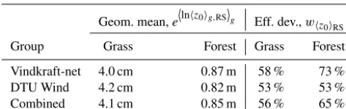
Table 2.Bootstrapped statistics of mean roughnesses from (resam-pled) user-providedz0given by two groups of wind resource ex-perts, using three resampled values per mean calculation; data are for the two terrain types shown in Fig. 2.
Geom. mean,e
lnhz0ig,RSg
Eff. dev.,whz0iRS
Group Grass Forest Grass Forest
Vindkraft-net 4.0 cm 0.87 m 58 % 73 % DTU Wind 4.2 cm 0.82 m 53 % 53 % Combined 4.1 cm 0.85 m 56 % 65 %
roughness lengths for the two cases is on the order of but larger than the expected roughness length itself, i.e., by a factor of∼1.1–1.3 times the estimated meanz0for grass or ∼1.1–1.6 times the mean for the forest case. This might be taken as an estimate for uncertainty inz0for such cases.
The variability in the user data differs between the polled groups and might be affected by the limited sample size. Due to the limited distributions of polled roughness lengths (not shown) gathered from each of the two expert groups, an al-ternate estimate of collective user uncertainty (i.e., industry-wide) is provided by again applying a resampling method to the distribution of surveyed z0. Following the averaging of expert-elicitedz0and the uncertainty characterization of the previous section, bootstrapping (Varian, 2005; Wu, 1986) is used to resample the elicited z0 values and construct a distribution of the means. Calculating each mean from n
nonunique random data samples and repeating 106times, we generate distributions ofz0 for the two cases. Forn&3, we find log-normal distributions for the bootstrapped geometric mean z0= hz0ig, as expected from the central limit theo-rem (lnz0becomes Gaussian). In the limit of the sample data set being perfectly representative of wind industry practices, the bootstrapped distribution for a givennis equivalent to the
P(z0) expected when any given wind engineer usesnvalues to calculate the mean roughness for a site such as the grass or forest case used here. The means of the resampled dis-tributions are the same as for the raw roughness samples in Table 1, regardless ofn. The deviation, however, decreases with n. For n=1, the deviations converge to those in Ta-ble 1, while the values of the effective geometric deviation
whz0iRS behave as approximately 1+n
−0.53 (the deviations
fall slightly more rapidly than n−1/2due to the slightly ir-regular sample or survey). As an example, Table 2 shows the geometric means and deviations for these mean distributions usingn=3 for the two groups and cases considered.
From Table 2, one infers the seemingly obvious result that for users taking an average of three industry-accepted rough-ness estimates (assuming that they span the sample taken) – instead of just one – the expected (industry-wide) uncertainty is reduced; we point out that such a conclusion depends on having reasonably representative roughness values to choose from.
To summarize, in this subsection we saw that the equiv-alent (normalized logarithmic) standard deviation from sur-veys of engineer or user-assigned roughness is of the order of the expected roughness itself, as shown in Table 1. In terms of Eq. (4), we expect an uncertainty equal to the half width of the (expected user input) distribution of lnz0to be approxi-matelywhz0ig∼ hz0ig. In the following section we would like
to show, in general, how uncertainty inz0– whether due to user input or measurement – propagates into wind speed and AEP estimates.
3.2 Propagation of roughness uncertainty
The uncertainty in roughness length has an effect on a num-ber of key variables needed for wind resource assessment. Since the geostrophic wind depends upon the surface fric-tion velocityu∗, in practice one must use a wind profile form (model) to translate measured wind statistics (e.g.,
Weibull-Aor mean wind speed) into the correspondingu∗analogue. This is typically accomplished by using the log law (Eq. 1), which is valid in statistically neutral conditions, and approx-imately in the mean (Kelly and Gryning, 2010; Kelly and Troen, 2016). Furthermore, to relateu∗at the prediction site to the (mean) geostrophic windG, Eq. (3) must somehow be solved foru∗. A direct analytical solution foru∗(G) via Eq. (3) is not possible; thus, Jensen et al. (1984) developed the approximate “reverse geostrophic drag-law” form
u∗(G)' 0.485G ln(G/f z0)−A0
. (5)
We adopt Eq. (5) and use it along with Eqs. (1) and (3) in order to relate wind speeds and roughness lengths for a given pair of prediction and measurement sites.
3.2.1 Sensitivity of predicted wind speed to background roughnesses
∂lnUpred ∂lnz0,1
' 1
ln(zobs/z0,1)
1− 1
ln[G/(f z0,2)] −A0 (6) × ( 1−
Uobs/G
ln(zobs/z0,1)
2
ln
κUobs
f z0,1
−A0 ln
zobs
z0,1
−1
)
and
∂Upred
∂lnz0,2 '
cGG
κ
A
0+ln zpredf/G
ln G/(f z0,2)−A02
. (7)
Here we have made the expression compact by writing
G(Uobs, zobs, z0,1) simply asG. Inspection of the two sensi-tivity expressions, Eqs. (6) and (7), reveals thatUpredis more sensitive to the background roughness at the observation site (z0,1) than the roughnessz0,2at the prediction site. Further-more, it is seen thatUpredalso has some sensitivity to obser-vation heightzobs, whilez0,1dominates.
From Eqs. (A1)–(A2), which follow from Eqs. (6)–(7) (see Appendix A for details), we arrive at an (implicit) expression relating the uncertainty in predicted hub-height wind speed to the uncertainty in background roughness at the observation site (1z0,1):
1Upred Upred
1z0,1
'exp
1.11+ zobs 80 m
−1/7
(8)
×hlin(zobs/a1z0,1)−1/7
o
−lin(z1/z0,1)−1/7
oi ,
where li(x) is the log-integral function (e.g., Abramowitz and Stegun, 1972; see appendix also). In Eq. (8), a1is the frac-tional uncertainty in observation-site background roughness length,
a≡z0+1z0 z0
=1+1z0/z0, (9)
evaluated atz0=z0,1. Thus, roughness uncertainties can be described geometrically (as they should be): for a given back-ground roughness, we then have a range of log roughness described by ln(z0,1)±ln(a) and corresponding roughness lengths ranging fromz0,1/atoaz0,1.
Just as Eq. (8) was derived above for variations in rough-ness at the measurement site, we similarly derive the un-certainty in predicted wind speed due to unun-certainty in the prediction-site roughnessz0,2from Eq. (7):
1Upred Upred 1z
0,2
' h
1− lna ln(zpred/z0,2)
i
h
1+ lna
A−ln[G/(f z0,2)]
i. (10)
This follows from Eq. (A3), which includes details of the derivation (Appendix A).
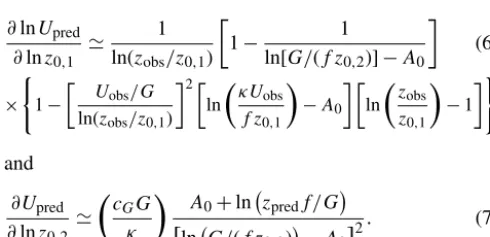
The sensitivity of hub-height (predicted) wind speed to
z0,1, via Eq. (8), is shown in Fig. 3 for the case ofzobs=60 m
observation height and a hub height of 100 m. Similarly, the uncertainty in predicted wind speed due to uncertainty in prediction-site roughnessz0,2, via Eq. (10), is displayed in Fig. 4.
The estimated relative uncertainty in predicted wind speed (1Upred) is first plotted vs. fractional roughness uncer-tainty a for a number of different measurement-site back-ground roughnesses (z0,mast), and then it is also plotted against z0,mast for different relative roughness uncertainty (1z0,mast/z0,mast=a−1), expressed as a percentage. For small background roughnesses one can see less effect on pre-dicted wind speed for a given roughness error or uncertainty, with a nearly linear dependence of relative wind speed uncer-tainty uponz0,mastfor measurements taken over smooth land or water (z0,mast<∼1 cm). For larger magnitudes of rough-ness uncertainty, as expected, one sees larger expected uncer-tainty in wind speed as well; this effect is reduced for smooth measurement sites (in conjunction with the previous state-ment). Also, for higher background roughnesses, the sensi-tivity of wind speed to (relative) roughness error is ampli-fied, as shown by the green lines in panel a or the right-most (highz0) part of panel (b) in Figs. 3–4. Comparing Figs. 3– 4, one also sees that the effect of a given change (or uncer-tainty in)z0,2has the opposite sign of the corresponding ef-fect due to an equal change inz0,1, but with the measurement or mast location’s roughnessz0,1having a larger effect than the prediction site roughnessz0,2. That is, the magnitudes of 1Upred(1z0,1) in Fig. 3 are larger than the magnitudes of 1Upred(1z0,2) displayed in Fig. 4.
Roughness bias and combined effect ofz0sensitivities at measurement and prediction sites
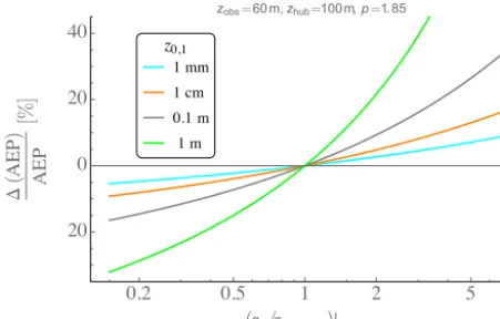
Above we saw that wind speeds predicted via the GDL (Eq. 3) with roughness-affected (logarithmic) wind profile (Eq. 1) can be more sensitive toz0,1than toz0,2. Thus, for an overall bias in roughness estimates, we should expect a net bias in wind speed predictions via wind atlas methods. In other words, for roughnesses that are systematically overes-timated (or underesoveres-timated) by the same factorabiasat mea-surement and prediction sites, we then expect a correspond-ing bias in predicted mean wind speed. This effect is shown by Fig. 5, which displays the fractional change in predicted wind speed as a function of fractional change in measure-ment and prediction-sitez0 for combinations of{z0,1, z0,2} that span typical application (colored lines).
As one might expect, for measurement and observa-tion sites with similar background roughness, the change
Figure 3. Error in predicted wind speed due to error in background roughness at measurement site via Eq. (8), for observation height zobs=60 m and prediction (hub) height ofzpred=100 m. (a)Error vs. ratio (=a) of estimated to actual backgroundz0. (b)Error vs.
backgroundz0at observation mast; uncertainties of{−67,−50,50,100,200}correspond toa=
n
1
3,12,1.5,2,3
o
.
Figure 4. Error in predicted wind speed due to error in background roughness at prediction site via Eq. (10), for observation height zobs=60 m and prediction (hub) height ofzpred=100 m. (a)Error vs. ratio (=a) of estimated to actual backgroundz0. (b)Error vs.
backgroundz0at observation mast; uncertainties of{−67,−50,50,100,200}correspond toa=
n
1 3,
1 2,1.5,2,3
o
.
abias. In addition to the typical range ofz0used in wind re-source estimation (colored lines), Figure 5 also shows the gross effect of measurement over forest (or effectively more complex terrain, i.e., with effective roughnessz0,1=1 m; de-noted by grey lines); one can see the corresponding increase in1Upred/Upredfor such cases when there is overestimation ofz0, even ifz0,2andz0,1are both 1 m.
In contrast to a possible bias in roughness assignment, one can imagine a worst case scenario as having a negative er-ror in z0,1 and a positive error inz0,2 (or vice versa), e.g., a1=1/a2. In this scenario the result resembles the plots in Fig. 5, but rotated 45◦with they axis stretched by a factor of 2: cases withz0,1=z0,2 no longer have small error, but all the lines show a large uncertainty for a far from 1 (e.g., ±40 % at a±11=a2∓1=0.1 forz0,1=1 cm and z0,2=1 m, corresponding to the solid green line), and all lines have
1Upred=0 fora=1.
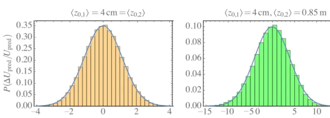
A more general situation is that of independent errors in roughness assignment at different sites. In this limit, one foresees a distribution of1Upred, given uncertainties inz0,2 and z0,1 (basically P(z0,2) and P(z0,1)). Two examples of this are given in Fig. 6. The figure showsP(1Upred/Upred) for the cases of winds observed over grass but predicting
winds over grass or forest, where the grass and forestz0have log-normal distributionsP(a) with means and widths given for the combined samples in Table 1. Following the earlier examples, the observation height is taken as 60 m and pre-diction (hub) height is 100 m.
In the figure, one can see the combined effect of different roughness distributions and uncertainties, particularly for the case of grass to forest (panel b in Fig. 6). For this case, the half width of the grassP(z0,1) corresponds to 117 % (where hz0,1i =4 cm) and that for the forest corresponds to 141 % of hz0,2i =0.85 m following Table 1. The combined effect gives wider error distributionsP(1Upred) for the grass-to-forest case than for the grass–grass case, as expected from Fig. 5, for example; the standard deviations corresponding to the z0-induced mean-wind error distributions in Fig. 6 are 1 and 4 % for the predictions over grass and forest, re-spectively (and both error distributions are nearly Gaussian, with skewnesses of 0.02 and −0.2). To be yet more con-servative, if we follow Sect. 2.1.2 using a gross estimate of observational z0 uncertainty equivalent to a half width (roughness uncertainty factor) ofwhz0iRS∼3, the uncertainty
considera-��� ��� � � � –��
–�� � �� ��
�����=(��/���������)
[
Δ
����� �����
]
����� ������
(%
)
����=��������= ��� ��
����=��������=���
����=��������=��
����= ���������= ��� ��
����= ���������=���
����= ���������=��
����=�������=���
����=�������=��
–
Figure 5.Total error in predicted wind speed due to a bias (abias) in background roughness at both prediction and measurement sites for different combinations of background roughness at the sites. As in Figs. 3–4, observation height iszobs=60 m and prediction (hub) height iszpred=100 m.
–� –� � � �
���� ���� ���� ���� ���� ���� ���� ����
�����/�����(%)
�
(
Δ
��
��
�
/
��
��
�
)
〈����〉=� ��=〈����〉
–�� �� � � � �� ��
���� ���� ���� ���� ���� ����
�����/�����(%)
〈����〉=� ���〈����〉=���� �
– –
(a) (b)
Figure 6.Distribution of error in predicted wind speed, given distributionsP z0,2/hz0,2i
, andP z0,1/hz0,1i
at prediction and measure-ment sites.(a)Prediction from grass to grass and(b)from grass to forest. InputP(z0) follows from elicited samples in Table 1; see text. Blue line is normal distribution based on calculated mean and standard deviation. As in Figs. 3–5,zobs=60 andzpred=100 m.
tion for wind engineers, we also point out that for predic-tion over water (again from zobs=60 tozpred=100 m with z0,1=4.1 cm) using the conservative roughness-uncertainty estimatea=whz0iRS∼3 again leads to uncertainty inUpred that exceeds 6 % and an error distribution that is somewhat non-Gaussian (skewness≈0.6, plot not shown); we provide this number to demonstrate the roughness-induced uncer-tainty expected when using land-based measurements for off-shore predictions.
3.2.2 Sensitivity of predicted energy production to backgroundz0
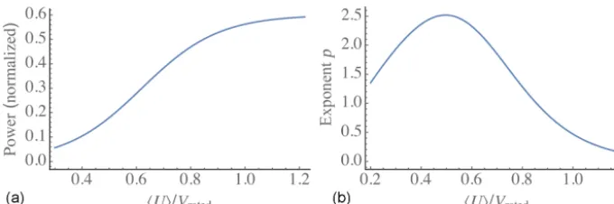
The uncertainty in background roughness can also be trans-lated into AEP uncertainty by employing a relation between wind speed and AEP, i.e., via a turbine (or perhaps wind farm) power curve. The propagation ofz0uncertainty to AEP follows that derived for wind speed above, but with some assumptions. First, we assume Weibull-distributed winds, which is standard practice in wind energy and also facili-tates analytical derivation of a bulk relation between AEP
and mean wind speedhUi. Because power curves in prac-tice do not have a “kink” at rated wind speed, but rather a smooth transition from the idealhUi3 regime to the maxi-mum (rated) power regime of operation (e.g., Wagner et al., 2011), we can derive an analytical effective power-curve form, expressible as a function ofhUi/Vrat, i.e., Eq. (B1) (shown in Appendix B). To accomplish analytical integra-tion and readily relate mean wind speed (or Weibull-A pa-rameter) per turbine-rated speed, some mathematical ap-proximations are used, wherein we also assume that the Weibull-k parameter is close to a value of 2 (within 10– 20 %). The analytical power-curve form PC(U/Vrat) then leads to a power-law relation between normalized AEP and wind speed: AEPnorm∝(hUi/Vrat)p, where the power-law exponentpis also a function ofhUi/Vrat, as shown in Ap-pendix B.
elu-����
� �� � ��
��� �
� �
��� ��� � � �
–��
� �� ��
(��/���������)����
Δ
(
���
)
���
[%
]
zobs=60 m,zhub=100m,p=1. 85
Figure 7.Sensitivity of (error in) predicted normalized power due solely to error in background roughness at measurement site vs. ra-tio of estimated to actual backgroundz0at observation mast (i.e., 1+relative error, Eq. 9) for various values of actualz0,1. Observa-tion height is 60 m and hub height is 100 m, as in Figs. 3–6.
cidated in Appendix B (see Fig. A4b). For Fig. 7 we con-sider the same situation as used for Figs. 3–5 (zobs=60 and zpred=100 m). As one might expect, the AEP uncertainty – due to uncertainties inz0,1,z0,2, or their combined effect with a common bias – simply resembles the wind speed un-certainty plots shown in Figs. 3–5: the vertical axis of the plot appears stretched by a factor of p('1.85). An analo-gous plot of the distribution of AEP error follows similarly; for a given value ofp(here 1.85), the horizontal (x-) axes in the plots of Fig. 6 are stretched by a factor ofp to give the distribution of1AEP.
3.3 Effect of uncertainty in background roughness upon wind resource predictions
In order to give examples (and realistic numbers) useful to wind engineers, in this section we translate the observation-based (Sect. 3.1.1) and user-observation-based (Sect. 3.1.2) roughness un-certainties into unun-certainties of predicted mean wind speed and AEP for the observation and user-survey examples treated in Sect. 3.1.1 and 3.1.2, respectively.
3.3.1 Uncertainty in predicted mean wind speeds
The relative uncertainties implied by roughness lengths cal-culated via surface-layer wind speed measurements were outlined in Sect. 3.1.1 for the seemingly ideal grassy terrain east of Høvsøre. The half widths of the roughness distribu-tions for the homogeneous sectors were found to be on the order of a factor of 3 timeshz0i, while the uncertainty in ob-taining a mean (representative) roughness was found through bootstrap resampling to be much smaller, about 5 %; this re-sult came whetherz0 was calculated from speeds at multi-ple heights in the ASL or from sonic anemometer measure-ments ofUandu∗in the ASL. However, despite similar
dis-tribution widths and similar apparent uncertainty in mean-estimation, thehz0ithemselves differed by roughly one-half order of magnitude, i.e., a factor of∼3 when determined in these two different ways. Thus, we first consider (conserva-tively) a relative uncertainty ofa∼3±1for z0, for the typ-ical resource-assessment heights (zobs=60,zpred=100 m) used in Figs. 3–7. As seen in Fig. 5, for systematic (bias) overestimates ofa≡1z0/z0and a mean roughness length at the observation site of 1 cm, this translates into wind speed uncertainty values of less than 1 % when predicting 100 m winds over the same roughness and gives 1Upred of {2,−2,−6,−10 %} for predictions over roughnesses of
z0,2= {0.2 mm, 3 cm, 30 cm, 1 m}. For the same magni-tude of systematic underestimate (a∼1/3) the correspond-ing1Upred/Upred are{−1,2,5,9 %}for thesez0,2, with an uncertainty of 1 % for 100 m winds predicted over the same roughness as the measurement site. Thus, we see about 1 % uncertainty inUpredfor these typical heights and the same ob-servation and prediction roughness. Meanwhile, using such observations to predict winds over nearby forested land, for example, incurs higher uncertainties, with magnitudes of 5– 10 %, without yet considering modeling the flow over such terrain. To get estimates of 1U(1z0) for other observa-tion and predicobserva-tion heights and roughnesses, we remind the reader that these can be obtained from Eqs. (8)–(10).
For the uncertainties inherent in user-provided roughness lengths, we address the two cases treated in Sect. 3.1.2. The grass case is similar to that considered in the Høvsøre anal-ysis above, with a mean roughness of about 4 cm. If we take the half width of the expected user-input distribution ofz0,
i.e., exp n
σln[z0/hz0ig]
o
from Table 1, then we can again ar-rive at estimates for the wind-speed uncertainty (this is also a bit conservative because it gives larger uncertainties than the bootstrap-derived half width). Again assuming typical appli-cation heights (zobs=60,zpred=100 m) for predictions over site roughnesses, z0,2= {0.2 mm, 1 cm, 30 cm, 1 m} and a z0-bias of 2.2±1 (±120 % from Table 1), we obtain Upred uncertainties of+{3,1,−3,−6 %}and−{2,0.4,−3,−5 %}. These roughly correspond to (a proxy of) the industry-wide uncertainty in predicted wind speeds (with thiszobs,zpred) for observations over a background roughness like the grass in Fig. 2. For the surveyed forest roughness in that figure, we get corresponding1Upredfollowing Table 1 for the case of all-site biases (±141 %→a≈2.4±1applied to bothz0,1 andz0,2). For predictions from observations over such a site, applied to turbine sites withz0,2={1 cm, 10 cm, 1 m} we get 1Upred≈(+){11,9,3 %} for systematic overestimates and (−){6,4,0.3 %}for systematicz0underestimation. The latter finding is rather significant as it implies that an underestima-tion of forest roughness lengths is safer than overestimating
meters there (Boudreault et al., 2015), industrial practice has been to usez0of 1 m or less (e.g., Troen and Petersen, 1989; Mortensen et al., 2014).
3.3.2 Uncertainty in predicted energy production
The magnitude of z0-induced AEP uncertainty for typical simple sites depends in general on the ratio ofhUi/Vrat (for classically behaved turbines) because the relationship be-tweenhUiand AEP depends on this ratio; this dependence is most simply expressed via the exponent
p=ln(AEP)
lnhUi for a power-law relation AEP= hUi
p, (11)
detailed in Appendix B. As mentioned in the previous sec-tion, with regards to uncertainty in the background rough-ness of either the observation or prediction site (or for a bias across both sites), the sensitivity plots of 1hUi per given roughness error are simply translated into analogous AEP-sensitivity figures via stretching the vertical axes by a factor
p(as was done to get Fig. 7 from Fig. 3a); similarly the hor-izontal (1U) axis in Fig. 6 is stretched by a factorp. Since
p basically varies between∼0.8 and 2.5 (over the reason-able range ofhUi/Vrat∼0.5–0.9), then the mean wind speed uncertainties quoted in the previous subsection can be sim-ply multiplied by a factor of∼0.8–2.5, depending on the ex-pected turbine power curve and subsequentp.
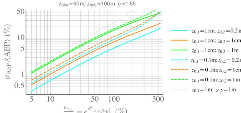
For most general practical use, we ultimately consider roughness error distributions and the consequent AEP error distributions, such as those shown in Fig. 6. For indepen-dent roughness error distributions at measurement and pre-diction sites, and assuming log-normal distributed 1z0 (as demonstrated in Sect. 3.1.1 and 3.1.2 for measured and user-estimated distributions), via Eqs. (8) and (10) we can ob-tain distributions of1AEP. The uncertainty inz0can be ex-pressed in terms of the dimensionless widthwz0/hz0i; for a given width we can synthesize distributions ofz0,1andz0,2, and then find the standard deviation of the resulting distribu-tion of1AEP. We do such Monte Carlo simulations over the range of dimensionless widths from 5 to 500 % for the same {z0,1, z0,2}pairs and observation and prediction heights as used in Fig. 5; the results are shown in Fig. 8.
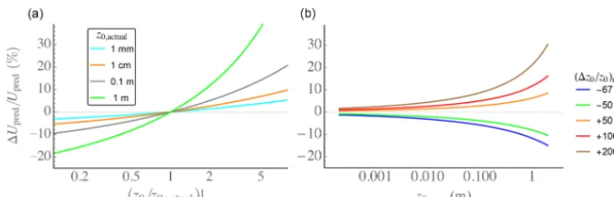
Figure 8 shows AEP uncertainty vs. roughness uncer-tainty; the latter is expressed as the dimensionless width
wz0/hz0i of the z0 distribution, calculated via the standard deviation of ln(z0/hz0i) as in Eq. (4). Following the previ-ous subsection’s analysis (wherezobs=60 m,zpred=100 m, and p=1.85), Fig. 8 shows that for actual measurement-site roughness z0,1≈1–10 cm, given a relative z0 uncer-tainty of 100 % (corresponding towz0∼z0as in Sect. 3.1.2), the GDL/z0-induced AEP uncertainty ranges from ∼5 % (for hz0,1i =1 cm, predicting over water) to 15 % (for hz0,1i =10 cm, hz0,2i =1 m). For the statistical uncertainty example of (mostly) homogeneous flat farm and/or grassland shown previously in Fig. 1 (Sect. 2.1.2), taking the relative
background roughness uncertainty factor to be equivalent to the width of the ln(z0) distribution (centered around∼1.4 cm for wind directions from∼45 to 120◦), i.e.,a∼3±1, leads to a similar AEP uncertainty range, roughly 6–16 % for pre-diction sites ranging from water to forest or urban. How-ever, such an uncertainty estimate seems large and may be explained considering Table 2. For industrial use, wind en-gineers (e.g., in medium or large companies) in effect assign a kind of ensemble-average roughness length for any given land-use type. Consider, for example, the case of taking three community-accepted values for the grass site as in Table 2, i.e., a relativez0 uncertainty of roughly 50 %, one can see from Fig. 8 that the AEP uncertainty drops to 4–10 %. One is reminded that these AEP uncertainty values correspond to the case of observation and prediction heights of 60 and 100 m, respectively: the slight dependence of1AEP onzobs andzpred modifies the uncertainty for other heights. Aside from the weak dependence on measurement and prediction heights, one also sees a basic power-law form emerging for the AEP estimates:
σAEP hAEPi ∝ ∼
w
z0
hz0i 6/7
, (12)
particularly for relative roughness uncertainties (widths of the distributionP(lnz0/lnhz0i)) that are
wz0/hz0i<∼1–2.
We also note again that we have focused here on the AEP uncertainty caused by uncertainty in background roughness rather than thez0uncertainty itself. Further details of the lat-ter are the subject of ongoing work and another paper, and here we point to Fig. 8 as the significant result: for a given uncertainty inz0, one can find the corresponding uncertainty in AEP due to use of the GDL–EWA method.
4 Conclusions
First we review the context of this work, i.e., the EWA method (Troen and Petersen, 1989)5, which employs the geostrophic drag law (Eq. 3) to perform horizontal extrapo-lation: mean wind speed measured at a site with some back-ground roughness(es) can be used to predict the mean wind at another location with potentially different surface character-istics, assuming the sites are forced by the same pressure gra-dient (geostrophic wind). For separate measurement and/or prediction sites where the EWA method is valid6, resource
5The EWA method is implemented in WAsP and related
soft-ware (e.g., windPRO, WindFarmer).
6The GDL applies to sites with approximately the same
�
��
��
���
���
���
�
�
��
��
��� 〈��〉
=
�
�
���
( %)
σ
���/
〈
���
〉
(
%
)
zobs=60m,zhub=100 m,p=1. 85
����=��������=��� ��
����=��������=���
����=��������=��
����=���������=�����
����=���������=���
����=���������=��
����=�������=��
Figure 8.Uncertainty in AEP vs. (relative) roughness uncertainty due to the combined effect of observation and prediction site roughness-uncertainty; independent log-normal roughness distributions assumed, with dimensionless widthwz0/hz0i. Standard deviation of AEP shown
for different combinations ofhz0,1iandhz0,2i. Case shown forp=1.85, i.e., AEP=U1.85as in Fig. 7.
assessments that account for background roughness length (z0) tend to be better than assessments that ignorez0 (such as those based only on observed shear exponent; see Kelly, 2016). This is especially true for sites in terrain with differ-ent background roughness; consequdiffer-ently, the EWA method has been used in wind energy for decades. The need for and justification of this method is also implied by Fig. 4, which displays the sensitivity of EWA-predicted winds to turbine-site roughness (z0,2); it can thus also be used to show how much the predicted mean wind changes due to z0,2 differ-ing from the measurement-site roughnessz0,1. Forz0,2/z0,1 deviating significantly from 1 (taking thex axis of Fig. 4a as this ratio), a significant1Upred can result, and the EWA method is needed to account for such. One can see that if
z0,2 differs from z0,1 by a factor of 5, the predicted mean wind may be affected by∼5–25 %; subsequently, the AEP could change by a factor of up to ∼2.5 times this, i.e., as much as∼60 %.
Using the EWA method, uncertainty in z0 leads to un-certainty in resource predictions that can be significant, as shown in Sect. 3. Both user-implicit (Sect. 3.1.2) and definition-related (Sect. 3.1.1) uncertainties in roughness length are found to effectively be (treatable as) roughly of the same order of magnitude, and they lead to an uncertainty in prediction of mean wind speed and AEP. The uncertainty in prediction is slightly more sensitive to measurement-site roughness z0,1 than prediction-site roughness z0,2, as seen in Eqs. (8)–(10) and displayed in Figs. 3–4. However, there is also a minor dependence on measurement and prediction heights via the vertical wind profile used within the EWA method (log law implicit in Eqs. 8, 10); shown by Fig. A2 in Appendix A.
As mentioned in Sect. 3.1.1, even in ideal (steady, neu-tral) conditions, the mean roughnesshz0iobtained from ob-servations and Eq. (1) via different calculation methods in the surface layer, such as using wind speeds at multiple heights or alternately wind speed with friction velocity, differs by an amount that appears to greatly exceed the uncertainty derived for any given method. For example, bootstrapped distribu-tions ofhz0i for the homogeneous flat grassland sectors at Høvsøre had relative widths (approximate uncertainty) well under 10 % when using Eq. (1) andUobsin the surface layer, whether calculated with or withoutu∗; however, the ratio of the means (or peaks ofP(hz0i)) from the different calcula-tion methods was roughly 3. In contrast, the uncertainty ofz0 estimated from polls of two groups of wind resource assess-ment experts (for grassland and forest) in Sect. 3.1.2 was on the order ofz0 itself, i.e.,w/hz0i ∼1 when estimated from single values ofz0 as in Table 1; such uncertainty shrinks, however, if assuming that wind engineers gauge roughness from a collection of accepted sources, as in the example of Table 2.
uncertainty in AEP (or scaled mean wind) predicted via the EWA method for a given uncertainty in background rough-ness length and pair of surface types (roughrough-nesses) at sepa-rate prediction and measurement sites. From Fig. 8 we see that the basic trend for uncertainty in mean wind speed or AEP behaves as approximately (w/hz0i)6/7 in the dimen-sionless roughness uncertainty regime w/hz0i<∼200 %, i.e., just within the range we have estimated.
There are other sources of uncertainty implicit in the use of the EWA method, in addition to the roughness lengths. Addi-tional uncertainties include the applicability of the GDL (see footnote 6), the constants (A, B) within Eq. (3), and the ac-tual form and/or use of Eq. (3) with arguments averaged in an ensemble (or spatial) sense. These are beyond the scope of the current paper. However, as for applicability of the GDL, regarding the distance between measurement and prediction sites, we remind the reader that (fine-resolution) mesoscale models give an indication of the spatial extent (and direction) of variations in the geostrophic wind, and we refer the reader to Hahmann et al. (2015) and Troen and Petersen (1989), for example. As to the distance over which one may horizon-tally extrapolate in more complex terrain, this depends upon the observation and prediction heights, along with the ter-rain complexity (as ruggedness index RIX, Mortensen et al., 2006, or local elevation variability Kelly et al., 2014a, Kelly, 2016); we point the reader to Clerc et al. (2012) and Troen et al. (2014) for uncertainty in complex terrain. The minor uncertainties due to GDL constants (A, B) are the subject of ongoing work (e.g., Floors et al., 2015), and the GDL aver-aging issue is currently seen to be secondary due to the well-behaved nature of Eqs. (8) and (10) and the magnitude ofz0 variations expected.
Additional uncertainties can also arise due to the use of a (mean) wind profile expression, such as the simple log law (Eq. 1) invoked here. One uncertainty is due to the appli-cability of a given profile model. Following Troen and Pe-tersen (1989) and due to the statistical dominance of neu-tral conditions (Kelly and Gryning, 2010), we have used the (surface-layer) form (Eq. 1) applicable in neutral conditions; furthermore, we limit our observational analysis to neutral steady conditions and observations to be within the surface-layer, where the logarithmic profile is valid and the roughness length is simply defined. However, deviations from logarith-mic may occur above the surface layer, such as for the pre-diction height considered in the figures (100 m), in the case of very shallow ABL depths (i.e., depths less than∼2zpred, Pedersen et al., 2014, or 200 m in this case) that occasion-ally occur (Liu and Liang, 2010). This ABL-depth effect is negligible for zpred close tozobs(andz0,1/z0,2 near 1) and is minor for the heights considered. However, an additional uncertainty dependent upon the ABL depth could be mod-eled following Kelly and Gryning (2010) and Liu and Liang (2010), or alternately a better profile form (e.g., Kelly and Gryning, 2010) could be invoked along with the GDL, par-ticularly to reduce uncertainties for predictions well above
100 m or in areas where lower-level jets are expected. An-other uncertainty arising implicitly from the profile model, as analyzed here, is due to considering the samez0for use in both the profile model and the GDL. That is, the wind profile reacts to a more local roughness, whereas the GDL reacts to a geostrophic-scalez0. In Troen and Petersen (1989) the latter is obtained by taking a weighted geometric spatial average ofz0, where lnz0is integrated upwind from a given location with a weighting function that decays with distance7; thus, the local and geostrophicz0 can differ slightly. This is not likely to have a major effect on the analysis here since the Høvsøre sectors considered were ideal and without signifi-cant inhomogeneity, such that the upwind-averaged rough-ness is within 10 % of the localz0. However, it is worth not-ing that for large roughness changes (e.g., coastlines) within ∼10 km upwind of a site, the geostrophicz0will differ from the site’sz0; Eqs. (8)–(10) can be recast for such. The effect on roughness uncertainty incurred through such spatial aver-aging is expected to be (much) smaller than the crude factor
w/hz0i ∼3 (200 %) found and presented above, though sys-tematic evaluation of this effect is still a subject of ongoing research. Analogously, the height-dependent effect of inho-mogeneities upon roughness (i.e., above the ASL) – in par-ticular its uncertainty – is also under study, but is expected to be minor for simple terrain.
Vertical extrapolation has not been treated explicitly here, though it is implicit in the vertical profile used to esti-mate u∗ from observed wind for use in the GDL. Such treatment, in conjunction with taking the profile rough-ness and geostrophic-scale roughrough-ness to be the same, is a choice that we have made to facilitate systematic modeling of roughness-induced uncertainty; thus, we have been able to estimate the effect of roughness, which occurs through both the wind profile (vertical extrapolation) and through in-vocation of the GDL (horizontal extrapolation). A separate model for the uncertainty in vertical extrapolation using a logarithmic-based profile (as in the EWA and popular wind software, e.g., WAsP), but without considering roughness uncertainty, is given in Kelly and Troen (2016) and Kelly (2016). Treating thez0-related uncertainties separately, per the geostrophic drag law and wind profile, is the subject of continuing work beyond the scope of the current article.
4.1 Applications and implications
In increasingly complex terrain, the actual surface rough-ness becomes less significant compared to terrain slope with regards to affecting the flow. However, for horizontal ex-trapolation, the aggregate effect of the (complex) terrain-induced drag leads to an increase in the effective
geostrophic-7The EWA roughness-averaging weighting function is
pre-scribed as exp(−r/`r), whereris the distance upwind,`ris a length
scale roughness (Beljaars et al., 2004; Kelly et al., 2014a). Thus, the geostrophic-drag and roughness uncertainty analy-sis given in this work can also be applied towards improved use of microscale models in complex terrain when horizontal extrapolation is involved. In particular, computational fluid dynamics solvers (e.g., RANS and LES), when employed us-ing different simulation domains for measurement and wind farm sites, are typically used to calculate terrain-induced flow perturbations (speed-up factors) at the respective sites. How-ever, for domains with different degrees of complexity (or potentially different resolutions) – and thus different large-scale drag – then the use of the geostrophic drag law (or any analogous empirical algorithm or method) demands that measured wind statistics must additionally be transformed properly, accounting for differences in the effective domain-scale mean roughness in the two domains (per wind direc-tion). Thus, uncertainty in characterizing the effective rough-ness due to terrain drag can be translated into a correspond-ing uncertainty in mean wind (or AEP) via the framework presented here. Alternately, for a given pair of (observation, prediction) sites, the uncertainty in mean wind prediction due to neglect of terrain drag can be estimated: a bias is intro-duced, whereby the effective geostrophic roughness is un-derestimated. From Fig. 5 one can see, for example, that for sites with the same effective roughness (complexity) of
z0,eff∼1 m and with an underestimation of 1 order of magni-tude (abias'0.1), a positive error1Upred∼2 % is incurred.
Another implication of this work applies to assessment in forested regions. Some work on characterizing profile-amenable roughness over forest (e.g., Bosveld, 1997; Tian et al., 2011; Boudreault et al., 2015) implies thatz0over for-est is larger than what has been typically assigned in wind resource assessment (i.e., z0>1, not z0.1), despite such underestimates being used for decades in the wind industry (Troen and Petersen, 1989; Mortensen et al., 2001; Emeis, 2013; Landberg, 2016). We now see an explanation for this looking at Fig. 5: systematic underestimation leads to smaller errors in wind speeds predicted via the EWA method com-pared to a positive bias onz0, particularly for typical appli-cation where both measurement and turbine sites are in high-roughness areas (dash–dot line in Fig. 5) such as forest.
The roughness sensitivity–uncertainty analysis developed here also has application to – and implications on – the treat-ment of mesoscale model output for use in microscale wind flow models. In so-called meso-to-microscale downscaling or wind climate generalization (Hahmann et al., 2013; Bad-ger et al., 2014), mesoscale wind output (or statistics of such) is treated in order to avoid “double-counting” of local surface-induced effects by the microscale model that have already been included in the mesoscale modeling. Addition-ally, the meso–micro downscaling procedure facilitates driv-ing of the microscale flow simulation with mean winds that are appropriate as per the roughness input to both the mi-croscale and mesoscale models, i.e., an effective geostrophic wind via the EWA method. Since any given planetary
bound-ary layer (PBL) scheme in a mesoscale model can react dif-ferently for a given model resolution, it may be necessary to scale input roughnesses used in the generalization procedure (Kelly and Volker, 2016). For (homogeneous ideal) output wind profiles from a particular PBL scheme and resolution, the ratio of profile-impliedz0to input z0 can be used with the analytic sensitivity relations developed herein to system-atically adjust the input roughness map and/or to scale the wind inputs to microscale models.
An additional application following from the roughness analysis herein – and consequently ongoing research – in-volves a limitation inherent in using a single characteris-tic (mean) roughness length. Due to the statischaracteris-tical nature of roughness and the significant width of measured rough-ness distributions (e.g., Fig. 1), an improvement would be to useP(z0) instead of meanz0in wind assessment and at-mospheric flow modeling, following the suggestion of Kelly and Gryning (2010). This becomes yet more significant (and complicated) considering that the width of P(z0) tends to depend on direction and vary from site to site, and it also involves correlations with other variables (e.g., stability; Zil-itinkevich et al., 2008). Given the limited applicability of the EWA method to time series (the GDL was not explicitly de-rived in a statistical mean sense), refined wind resource es-timates – which are essentially statistical atmospheric fluid mechanics – using (joint) distributions of roughness and sta-bility offer potential improvement over current mean meth-ods and are a subject of continued study.
One final application follows from the analytical form introduced here to approximate common production power curves, in a general or universal way under the assumption of Weibull-distributed wind speeds. From this, the exponent in the power-law expression relating annual energy produc-tion and mean wind speed was derived, allowing us to relate uncertainty in roughness length to uncertainty in AEP. More flexible power-curve forms can also be made from logistic functions (e.g., generalizing those of Villanueva and Feijoo, 2016) as well. Regardless of the exact form, such analytical treatment also facilitates quick computation of power for a given set of Weibull parameters, which is applicable to large data sets such as the Global Wind Atlas (Badger et al., 2015). Lastly we re-iterate that issues in the definition of rough-ness length, and specific limits of its validity, are beyond the scope of this article. However, current ongoing work includes closer examination of the (turbulent) mechanisms involved in the observation of roughness length from wind measure-ments and heterogeneity; subsequent links to refined uncer-tainty characterization may follow such investigation.
4.2 Summary of conclusions and implications
– Uncertainty inz0leads to uncertainty in predicting re-sources using the EWA method.
– Uncertainty in EWA-predicted mean wind depends uponwz0, and to a lesser extent also upon{z1, z2}.
– wz0 (half-width of P(z0)) is of the same order as the mean, i.e., wz0∼ hz0i for both user- and observation-derivedz0.
– For modest z0 uncertainties wz0.2hz0i
, the
uncer-tainties{1U, 1AEP} ∝wz0/hz0i
6/7 .
– In complex terrain and/or forest, ignoring the effect of form drag causes a positive bias in predictions.
– Underestimation of aggregate forest roughness leads to smaller error than overestimation.
– Analytical form for power curve PC(U/Vrat) gives AEP(hUi) and thus uncertainty in AEP, i.e.,
1AEP(1hUi).
– EWA–GDL sensitivity expressions are applicable to treatment of WRF output for wind resources.