Damage Detection in Beam-like Structures Applying Finite Volume Method

(1)

DOI: 10.22075/jrce.2017.10599.1170

journal homepage: http://civiljournal.semnan.ac.ir/

Damage Detection in Beam-like Structures applying

Finite Volume Method

B. Mohebi1*, A.R. Kaboudan2 and O. Yazdanpanah2

1. Assistant Professor, Faculty of Engineering, Imam Khomeini International University, Qazvin, Iran 2. Ph.D. Student, Faculty of Engineering, Imam Khomeini International University, Qazvin, Iran

*

Corresponding author:[email protected]

ARTICLE INFO ABSTRACT

Article history:

Received: 18 February 2017

Accepted: 09 July 2017 In this article, a damage location in beamlike-structure is determined using static and dynamic data obtained applying the finite volume method. The modification of static and dynamic displacement due to damage is applied to establish an indicator for determining the damage location. In order to assess the robustness of the proposed method for structural damage detection, three test examples including static analysis, free vibration analysis and buckling analysis for a simply supported beam having a number of damage scenarios are taken into account. The acquired results demonstrate that the method can accurately locate the single and multiple structural damages in considering the measurement noise. Finite volume method results provided in this study for finding the damage location is compared with the same indicator derived via finite element method in order to evaluate the efficiency of FVM. The acquired results are indicated a good match between both the Finite Volume method and Finite Element method, and there are rational correlations between them.

Keywords: Damage Detection,

Static and Dynamic Noisy Data, Finite Volume Method,

Buckling Analysis,

Displacement Based Indicator.

1. Introduction

Local damage may occur during the lifetime of structural systems. On that account, a rehabilitation process is essential to increase the lifetime of the damaged system. Hence, finding the damage location is the main object before doing any rehabilitation process. Health monitoring is a process which leads to finding the local damage in

(2)

been introduced to determine the location and extent of eventual damage in the structural systems. In recent years many efforts have been performed to introduce new techniques for finding damage locations in structural systems. One of these techniques is based on the changes in vibration characteristics of the damaged system like modifications in natural frequencies which can be found in [1-2]. Many structural systems may experience some local damage during their existence. If the local damage is not identified timely, it may cause an unwanted outcome. Consequently, damage identification is an essential issue for

structural engineering, and it has received

considerable attention during the last years [3-4]. Structural damage detection consists of

four different levels [5]. The first level

determines the presence of damage in the structure. The second level includes locating the damage, while the third level quantifies the severity of the damage. The final level applies the information from the first three steps to estimate the remaining service life of the damaged structure. After discovering the damage occurrence, damage localization is more important than damage quantification. Attributed to a great number of elements in a structural system, properly finding the damage location has been the main concern of many studies. In the last years, numerous methods have been proposed for accurately

locating structural damage. Structural

damage detection by a hybrid technique consisting of a grey relation analysis for damage localization and an optimization algorithm for damage quantification has been proposed by He and Hwang [6]. Yang et al. applied an improved Direct Stiffness Calculation (DSC) technique for damage detection of the beam in beam structures. In their research, a new damage index, namely

Stiffness Variation Index (SVI) was proposed based on the modal curvature and bending moments using modal displacements and frequencies extracted from a dynamic test, and it was indicated that this damage index is more accurate in comparison to most other indexes [7]. Damage identification methods based on applying the modal flexibility of a structure were utilized by [8-11]. Techniques based on frequency response functions (FRFs) of a system were adopted by [12-14].

Damage identification based on Peak Picking Method and Wavelet Packet Transform for Structural Equation has been used by Naderpour and Fakharian [14]. In this paper, a two-step algorithm has been proposed for the identification of damage based on modal parameters. Results indicate that this preprocessing step causes noise reduction and lead to more accurate estimation. Moreover, investigating the effect of noise on the proposed method revealed that noise has no great effect on results. Moreover, for estimation damage locations and also the severity of the damage, two separate optimization procedures have been used [15].

A two-stage method for determining

structural damage sites and extent applying a modal strain energy-based index (MSEBI) and particle swarm optimization (PSO) has

been proposed by Seyedpoor [16]. An

efficient method for structural damage localization based on the concepts of flexibility matrix and strain energy of a

structure has been suggested by Nobahari

and Seyedpoor [17]. An efficient indicator for structural damage localization applying the change of strain energy-based on static noisy data (SSEBI) has been proposed by

Seyedpoor and Yazdanpanah [18]. The acquired results clearly illustrate that the proposed indicator can precisely locate the

(3)

developed for structural damage detection have been founded on using dynamic information of a structure that can be obtained slowly and expensively. However, the methods of structural damage detection employing static data are comparatively fewer, while static information can be obtained more quickly and cheaply. Finite volume method (FVM) is a popular method in fluid mechanics problems analysis, and it is rarely used in solid mechanics problems analysis. There is not any investigation on damage detection of structures applying finite volume method, yet some works have been done to indicate the efficiency of the method in the analysis of structures. The accuracy of the finite volume method in bending analysis of Timoshenko beams under external loads was investigated in [19]. In this paper, the accuracy of the finite volume method was examined in some benchmark tests. It was illustrated that shear locking would not happen in thin beams while this happens in bending analysis of thin beams applying the finite element method. This is a drawback of the finite element method which can be eliminated using some techniques like reduced integration. The application of finite volume method in calculation of buckling load and natural frequencies of beams is found in [20]. The method has been utilized in the analysis of very thin and thick beams in some benchmark tests to indicate the robustness of the finite volume method. All the results were in good agreement with respect to the analytical solution, and again, shear locking was not observed in very thin beams. THE FVM has been applied by Wheel [21] for plate bending problems based on Mindlin plate theory. In that work, the results have been obtained for thick and thin square and circular plates, which revealed that shear locking does not appear in the thin

plate analysis. The effect of mesh refinement was investigated in that work as well.Simultaneously, FVM based on cell-centered and cell-vertex schemes for plate bending analysis has been utilized by Fallah

[22]. In that work, some test cases have been examined for beams and square plates. The accuracy of the results has been compared with the conventional FEM to show the efficiency of FVM. He also presented the same conclusions about shear locking not happening in the analysis of thin beams and thin plates. More studies of utilizing finite volume method in solid mechanic problems can be found in [23] (about dynamic solid mechanics problems), [24] (about large strain problems), [25] (about dynamic fracture problems) and [26-28].

In this study, an efficient method applying finite-volume theory is introduced to estimate the damage locations in a structural system. The change of static and dynamic displacement between healthy and damaged structure has been used to form an index for damage localization. Various test examples are selected to assess the efficiency of the index for accurately locating the damage. Numerical results indicated that the method based on finite volume analysis could also identify the defective elements in a damaged structure rapidly and precisely compared with those of a finite element method (FEM).

2. The

Finite

Volume

(FV)

Procedure

(4)

2.1. Static Analysis

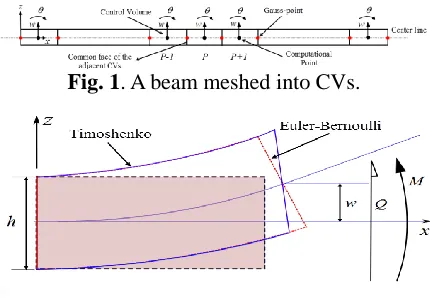
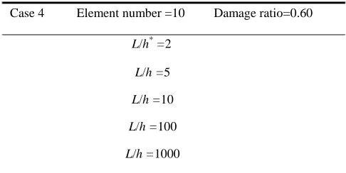
Fig. 1 presents a part of a beam meshed into 2-node elements accompanying the centerline of the beam, which is considered as the control volumes (CVs) or cells. Centers of the CVs are taken into account as the computational points where the unknown variables will be computed at these points. So a cell-centered scheme is utilized in the analysis. For each cell, the acting resultant bending moments and shear forces are evaluated at gauss-points located on cell faces, see Fig. 1. to obtain the beam governing equations, Timoshenko beam theory and small displacements assumption are applied , so shear deformations are included in the formulation derivation (as shown in the Fig. 2). is the transverse displacement and is the rotation of the CVs.

Fig. 1. A beam meshed into CVs.

Fig. 2. Deformation of a Timoshenko beam (blue) compared with that of a Euler-Bernoulli

beam (red).

The finite volume formulations are based on the conservation of the forces in each CV. Consequently, the equilibrium equation for cell P under uniform load (

q

) and concentrated loads (F_k ) can be written by computing the forces at the right (R) and left (L) side of the control volume, as indicated in the Fig. 3.

Fig. 3. Resultant forces of a CV under external forces.

,

. .

1

0 [ ( )]

( ) 0

p i i i i i p

i L R n o f

k k P k

M M n Q n x x

F x x



    

 



(1)

,

. .

1

0 [ ( )]

0

z i i i i p

i L R n o f

k k

F Q n qn x x

F



    





(2)

The first equation is the equilibrium of moments about the center of the CV, and the second one is the equilibrium of forces in

z

direction. M_i and Q_iare the bending moments and shear forces at the i th face of the CV respectively, x_pis the distance of the center of the control volume from the origin, x_kdenotes the location of the concentrated applied load F_k and n_i is the cosine direction of outward normal of the face.

When i L, n_i cos(180 ) 1 and when ,

i R n_i cos(0 ) 1 . The bending moments and shear forces at the i th face can be related to transverse displacements and rotations as follows:

( ) , . . ( )

i i i s i

d dw

M EI Q k A G

dx dx

 _

  

(3)

(5)

which is equal to 5 / 6 for a rectangular section, A is the area of the section and G is the shear modulus. Bending moment and shear forces are calculated based on the transverse displacements and rotations of the gauss-points. In the cell-centered approach, the unknown variables of the CVs are located at the centers of the CVs. So it is essential to make a relation between the unknown variables of the gauss-points and the corresponding unknown variables of the cell centers. For this purpose, a temporary 2-node isoparametric line element is applied . The temporary element nodes are located at the two adjacent cell centers as depicted in Fig. 4.

Fig.4. Temporary element in (a) global coordinate system, (b) natural coordinate system.

i

r at any point can be calculated as below:

1 12 2( ) 1 i i x x r l    (4)

Using the shape functions defined by the application of the temporary element, the transverse displacements and rotations of the gauss-points can be related to the corresponding values at the centers of the CVs.

2

1 1 2 2

1 2

1 1 2 2

1

i i i

w N w N w N w

N N N

           



(5) 1 2 1 1 2 2 r r

N   N  

(6)

1

N and N₂ are the shape functions at node 1 and 2 of the temporary elements in the natural coordinate system. Derivatives of the unknown variables can be calculated applying the chain rule law as below:

2

1 2

2 1 12

1 ( ) , 2 2 i i i i i i dN

d d dr dr

dx dr dx dr dx

dN x x l

dx x dr dr   _        



(7) 2 2 1 1 1

2 1 2 1

2 1 12

( i )( i )

i i

dN dN

d

x

dx dr dr

x x l

 _           _  



(8)

The same procedure is done for w. So:

2 1 12 w w dw dx l   (9)

Accordingly, the unknown variables and their derivatives for the right and left side gauss-points with neighboring CVs P 1,Pand

1

P can be written as below:

1 1 ( , ) ( , ) ( , ) , 2 ( , ) ( , ) ( , ) 2 P P R P P L w w w w w w             (10) 1 1 1 1 ( , ) ( , ) ( , ) [ ] , ( , ) ( , ) ( , ) [ ] P P R P P P P L P P w w d w

dx x x

w w

d w

dx x x

                (11)

(6)

kinds of boundary conditions can be presumed :

a. Displacement boundary conditions

b. Force boundary conditions

c. Mixed boundary conditions

Fig.5. Point cells bc1 and bc2 used for applying boundary conditions.

In case of displacement boundary condition, the transverse displacements and rotations should be equal to the corresponding value at the boundaries.

* *

1 1 1

* *

2 2 2

( , ) ( , )

bc bc bc

w w

 



 (12)

Moreover, in the case of force boundary condition, the bending moments and shear forces should be equal to the corresponding values at the boundaries.

* *

1 1 1

* *

2 2 2

( , ) ( , ) ,

( , ) ( , )

bc bc bc

M Q M Q



 (13)

And in case of mixed boundary conditions, an appropriate selection of the above equations is utilized for applying boundary conditions.

If ( , ,w



M Q, )_bci 0 one can write:

( , )w



_bci 0

(14)

1 1

1

1 1

( ) 0 0,

. . ( ) 0

0

bc bc

bc

s bc

bc bc bc

d EI

dx l

dw k A G

dx w w

l

  





  

 



  

(15)

2 2

2

2 2

( ) 0 0 ,

. . ( ) 0

0

bc n bc

bc

s bc

bc n bc bc

d EI

dx l

dw k A G

dx

w w

l

 





  

 



  

(16)

By assembling the equilibrium equations written for the CVs and equations expressing the boundary conditions obtained by applying point cells, the discretized governing equations of the beam can be expressed as follows:

2(n 2) 2(n 2) 2(n 2) 1 2(n 2) 1

K _{ } _ u _{ } F _{ }

(17)

Where n is the number of CVs, K is a matrix Containing the coefficients associated with the unknown variables, uis the displacement vector defined by Eq. 18 and F is a vector containing the load values acting on the cells and also the known values of the boundary conditions.

(18)



1 1 2 2 . . . 1 1 2 2



T n n bc bc bc bc

u  w  w  w  w  w

Applying the above equations and assuming

(7)

11 12 13 14 15 16

21 22 23 24 25 26

1 1 1 1 ( ) ( ) ( ) ( ) ( ) ( ) ( ) ( ) ( ) ( ) ( ) ( )

i i i i i i

i

i i i i i i

i i i i i i i

k k k k k k

K

k k k k k k

w u w w                                    (19) 11 12 13 14 15 16 . . . . . ( ) , ( ) , 4 2 . . . 2

( ) , ( ) 0,

2 . . . . . ( ) , ( ) 4 2 s s i i s i i s s i i

k A G l k A G

EI

k k

l

k A G l EI

k k

l

k A G l k A G

EI k k l            (20) 21 22 23 24 25 26 . . ( ) , 2 . .

( ) , ( ) 0

2 . .

( ) , . . . . ( ) , ( ) 2 s i s i i s i s s i i

k A G k

k A G

k k

l k A G k

l

k A G k A G

k k l         (21)

The same procedure can be done to calculate the matrix K_bc₁ and K_bc₂. For a simply supported beam at both ends the sub-matrix

1 bc

K and K_bc₂ are written as follows:

11 1 12 1 13 1 14 1 15 1 16 1

1

21 1 22 1 23 1 24 1 25 1 26 1

1 1 1 1 1 2 2 ( ) ( ) ( ) ( ) ( ) ( ) ( ) ( ) ( ) ( ) ( ) ( )

bc bc bc bc bc bc

bc

bc bc bc bc bc bc

bc

k k k k k k

K

k k k k k k

w u w w                                (22)

11 1 12 1

13 1

14 1 15 1

16 1 . . . 2 ( ) , ( ) . . , 2 . . . 3 ( ) 4 . . . . . ( ) , ( ) , 2 4 . . ( ) 2 s

bc bc s

s bc s s bc bc s bc

k A G l EI

k k k A G

l

k A G l EI

k

l

k A G EI k A G l

k k

l k A G

k             (23)

21 1 22 1

23 1

24 1 25 1

26 1

2 . .

( ) . . , ( ) ,

. .

( ) ,

2

3 . . . .

( ) , ( ) ,

2 . .

( )

s

bc s bc

s bc s s bc bc s bc

k A G k k A G k

l k A G

k

k A G k A G

k k

l k A G k l         (24)

11 2 12 2 13 2 14 2 15 2 16 2

2

21 2 22 2 23 2 24 2 25 2 26 2

1 1 2 2 2 ( ) ( ) ( ) ( ) ( ) ( ) ( ) ( ) ( ) ( ) ( ) ( )

bc bc bc bc bc bc

bc

bc bc bc bc bc bc

n n n bc n bc bc

k k k k k k

K

k k k k k k

w u w w                                  (25)

11 2 12 2

13 2

14 2 15 2

16 2 . . . . . ( ) , ( ) , 4 2 . . . 3 ( ) , 4

. . 2 . . .

( ) , ( ) , 2 2 ( ) . . s s bc bc s bc s s bc bc bc s

k A G l k A G EI

k k

l

k A G l EI

k

l

k A G EI k A G l

k k

l k k A G

  

  

  

 

(26)

21 2 22 2

23 2

24 2

25 2 26 2

. . . . ( ) , ( ) , 2 . . ( ) , 2 3 . .

( ) ,

2 . . ( ) . . , ( ) s s bc bc s bc s bc s

bc s bc

k A G k A G

k k

l k A G

k

k A G k

l

k A G k k A G k

l          (27)

(8)

2.2. Free Vibration Analysis

By modifying the static equilibrium equations (1) and (2) and taking into account the effect of mass moment of inertia and mass of the CVs, dynamic equilibrium equation of a beam in the absence of external load can be written as follows:

,

0

[ ( )] 0

p P

i i i i i p i L R

M j

M n Q n x x





   

  



(28)

,

0 0

z P i i

i L R

F m w Q n



    



(29)

p

m is the mass of the CV and j_p is the mass moment of inertia about the axis passing through the center of the CV and normal to the section of the beam.

In the same manner, as explained for static analysis, the governing equation of the free vibration of the beam can be written in the form of Eq. 30.

2(n 2) 2(n 2) 2(n 2) 1 2(n 2) 2(n 2) 2(n 2) 1 0

M _{ } _ u _{ } K _{ } _ u _{ }  (30) u is the acceleration vector which can be written as blew:

1 1 2 2 . . . 1 1 2 2

T

n n bc bc bc bc

u  w  w  w  w  w _

(31)

M is the mass matrix and for the i th internal CV the mass matrix, M_i , is defined by Eq. 32.

0

0 . .

pi i

i

j M

A l





 

  _ 

  (32)

pi

j is the mass moment of inertia of the

i th CV,  is the density, Ais the area of the section and li is the length of the i th

CV.

As boundary cell points are utilized for applying boundary conditions and have no mass, so a small value should be taken into account at the diagonal elements of M_i for boundary point cells. So:

1, 2

0 0

bc bc

a small value M

a small value

 

  

  (33)

By assuming the displacement vector in the form of Eq. 34 in free vibration of the beam and substituting Eq. 34 in Eq. 30 the free vibration governing equation can be written as Eq. 35.

ˆ cos

u u t ₍₃₄₎

2

ˆ ˆ

Ku  Mu ₍₃₅₎

 is the frequency vector. Eq. 35 is a standard eigenvalue equation. By solving this equation, the frequencies and mode shapes of the beam can be obtained.

2.3. Buckling Load Analysis

In the presence of axial forces, N , the modified form of the Eqs. 1 and 2 can be written as follows:

,

. .

1

0 [ ( )]

( ) 0

p i i i i i p

i L R n o f

k k P k

M M n Q n x x

F x x 



    

 



(36)

, . .

1

0 [ cos ( ) sin ]

0

z i i i i i p i i

i L R

n o f

k k

F Q n qn x x Nn

F

 



     





(9)

By postulating that small deformation assumption and with respect to Fig. 6, the following equations can be written.

Fig 6. Control volume P deformation due to axial loading.

cos i 1 , sin i ( )i dw

dx

   

(38)

By assembling the K_i matrix and F_i vector of each element, and applying the boundary conditions using point cells, the governing equation of the system is acquired.

2(n 2) 2(n 2) 2(n 2) 1 2(n 2) 1

K _{ } _ u _{ } F _{ }

(39) By solving the above equation, the unknown displacement vector can be obtained.

2.3.1. Calculation of Buckling Load

Eq. 39 can be written in the form of Eq. 40.

11 12 1

21 22 2

K K F

K K w F



    



    

 

   (40)

Using the first equation of Eq. 40 one can write:

1

11 12 1 11[ 1 12 ]

K K w F   K F K w

(41)

12

K can be written as a sum of the two matrices K and K .

12

K K NK

(42) Applying Eqs. 41 and 42 one can write:

1

11[ 1 ( ) ]

K F K NK w

 _  _ _

(43) The above equation can be substituted in the second equation of Eq. 40 to postulate Eq. 44.

1

21 11 1

22 2

1

21 11

1

22 2 21 11 1

[ ( ) ]

K K F K NK w K w F

K K K NK w K w F K K F



  



   

 

(44)

Eq. 44 can be represented as follows:

1 1

22 21 11 21 11 1

2 21 11 1

[(K K K K) N K K K w( )]

F K K F

 



  

 (45)

To calculate the buckling load, the determinant of the above equation should be equal to zero. By doing so, the below equation is.

1 1

22 21 11 21 11

(K K KK)N K K( K) 0 (46) Eq. 46 can be simplified in the form of Eq.

47.

0

C NC 

(47) By solving the above eigenvalue problem, the buckling load of the beam can be acquired .

(10)

In this paper, damage detection of a prismatic beam with a specified length is studied. First, the beam is divided into a number of CVs. Then, mode shapes of the healthy beam in measurement points are evaluated applied the finite volume method. As mentioned before, in cell-centered scheme computational points are located at the centers of the CVs. Towards a comparison with the finite element results, the deflections are interpolated at the element faces (element nodes) to acquire the corresponding values. A MATLAB (R2014b) code is prepared here for this purpose. Henceforward, consider the nodal

coordinates (xq ,q1 ,2 ,...,n1_{) and} _i_th

mode shape (h(q,i) ,q1 ,2 ,...,n1₎

obtained for the healthy beam as follows:

( , ) 1 (1, ) 2 (2, ) 1 ( 1, )

, ( , ), ( , ), . . ., ( , )

q h q i h i h i n h n i

x x x x_ _

       

   (48)

This process can be repeated for the damaged beam as well. It should be noted; it is assumed that the damage decreases the stiffness, and consequently, it can be simulated by a reduction in the modulus of elasticity (E) at the location of the damage. In this paper, it is supposed the damage occurs in the center of an element. So, consider the nodal coordinates and i-th mode shape (

1 ..., , 2 , 1 ,

) ,

(  

_d _q_i q n

) obtained for the damaged beam as below:



x_q,_d₍_q_,_i₎

 

 (x₁,_d₍₁_,_i₎),( x₂,_d₍₂_,_i₎),. . .,( x_n_₁,_d₍_n_₁_,_i₎)



(49)

Finally, applying the dynamic responses (mode shapes displacement) obtained for two above states, an indicator introduced in the literature is used here as [28-29]:

( , ) ( , ) 1

( )

nm

q i q i i

h

q

d

MSBI

nm



  





(50) Where nm is the number of mode shapes considered.

For static data, the Eq. 50 can be postulated

as below

( ) ( ) q d q yhq DBI y 

(51) Presuming that the set of the MSBI of all points (MSBIq , q1, 2,...,n1 ) represents a

sample population of a normally distributed variable, a normalized form of MSBI can be defined as follows:

mean( )

max 0 , ,

std( )

1, 2,..., 1

q q

q

MSBI MSBI

nMSBI

MSBI

q n

   

  _ _

 _ _

 

 

(52)

where MSBIq is defined by Eq. 49.Moreover,

mean (MSBI) and std (MSBI) represent the mean and standard deviation of (

1 ,..., 2 , 1 ,

q q n

MSDBI ), respectively.

mean( )

max 0 , ,

std( ) 1, 2,..., 1

q q

q

DBI DBI

nDBI

DBI

q n

   

  _ _

 _ _

 

 

(53)

In this paper, the results of the FVM based indicator given by Eqs. 52 and 53 are compared with the obtained results of FEM.

4. Numerical Examples

(11)

analysis, and free vibration analysis of FVM have been considered for a simply supported beam as presented in Fig. 7.

Fig 7. Geometry and cross-section of the simply supported beam.

4.1. First Example: Static Analysis

The simply supported beam with uniformly distributed load q 1kN /m depicted in Fig. 7 is selected as the first example. The beam is discretized by twenty 2D-beam elements leading to 44 DOFs. In order to assess the efficiency of the indicator given by Eq. 53, four different damage cases listed in Tables 1 and 2 are taken into account. It should be noted that damage in the damaged element is simulated, hereby reducing the modulus elasticity (E) at the damaged location.

Table 1. Four different damage cases induced in the simply supported beam

Case 1 Case 2 Case 3

Element number

Damage ratio*

Element number

Damage ratio

Element number

Damage ratio

2 0.80 7 0.60 10 0.80

- - - - 15 0.80

*Damage ratio is d

h

E E

Case 4

Element number Damage ratio*

17 0.80

- -

*Damage ratio is d

h

E E

Table 2. A damaged case induced in a simply supported beam having different (L/h)

Case 4 Element number =10 Damage ratio=0.60

L/h* =2

L/h =5

L/h =10

L/h =100

L/h =1000

*where L is the span length and h is the thickness of the beam

4.1.1. Damage Identification Without

Considering Noise

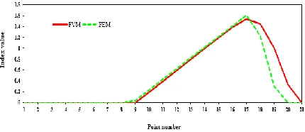
Damage identification charts of the simply supported beam in static analysis for cases 1 to 4 are illustrated in Figs. 8-12, respectively. As shown in the figures, the maximum value of the calculated indicator is located in the vicinity of the damaged elements. In addition, to verify the indicator given by Eq. 53., the result of FVM has been compared with that of FEM. As it’s depicted in the figures, the finite volume method is reasonably efficient as well as the finite element method in determining the damage location of the damaged element.

Fig 8. Damage identification chart of the 20-element beam for damage case 1 including FVM

(12)

and FEM damage based index

Fig 12. Damage identification chart of 20-element beam for damage case 4 considering: (a)

L/h =2, (b) L/h =5, (c) L/h =10, (d) L/h =100 and (e) L/h =1000

4.2. Second Example: Free Vibration Analysis

The second example is a simply supported beam with the same properties and geometry, as illustrated in Fig. 7. The density of the beam is ρ=1000 kg/m3. The beam is discretized by forty 2D-beam elements leading to 84 DOFs. In order to assess the efficiency of the indicator given by Eq. 52, four different damage cases listed in Table 3 are contemplated. It should be noted that damage in the damaged element is simulated, hereby reducing the modulus elasticity (E) at the damaged location.

Case 1 Case 2 Case 3 Case 4

Element number

Damage ratio

Element number

Damage ratio

Element number

Damage ratio

Element number

Damage ratio

14 0.70 8 0.70 12 0.70 9 0.70

- - 33 0.70 18 0.70 15 0.70

- - - - 28 0.70 23 0.70

- - - 29 0.70

- - - 36 0.70

*Damage ratio is d

h

(13)

4.2.1. Damage Identification Without Considering Noise

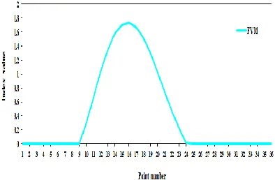
Damage identification charts of the simply supported beam in free vibration analysis for cases 1 to 4 are presented in Figs. 13-16, respectively. As shown in the figures, the value of FVM is further in the vicinity of some elements that this indicates, damage occurs in these elements.Moreover, for verifying the indicator given by Eq. 52, the result of FVM has been compared with that of FEM. As it’s presented in the figures, the efficiency of the proposed method for damage localization is high when compared with the damage indicator based FEM method.

Fig 13. Damage identification chart of the 40-element beam for damage case 1 considering: five modes for FVM and one mode for FEM

based index

Fig 14. Damage identification chart of the 40-element beam for damage case 2 considering: five modes for FVM and one mode for FEM

based index

Fig 15. Damage identification chart of the 40-element beam for damage case 3 considering: nine modes for FVM and three-mode for FEM

based index

Fig 16. Damage identification chart of the 40-element beam for damage case 4 considering: twelve modes for FVM and eight modes for FEM

based index

4.2.2. The Effect of Measurement Noise

In this part, the effect of measurement noise has been studied. For this instance , 3% noise is reviewed in scenario 4 of Table 3. As shown in Fig. 17, there is good compatibility between both damage identification charts with and without noise. In other words, the noise has a negligible effect on the performance of FVM.

Fig 17. Damage identification chart of the 40-element beam for damage case 4 considering 3%

(14)

4.3. Third Example: Buckling Analysis

The simply supported beam illustrated in Fig. 7 is selected as the third example for buckling analysis. The beam is discretized by thirty-five 2D-beam elements leading to 74 DOFs. In order to assess the efficiency of the indicator given by Eq. 52, four different damage cases listed in Table 4 are contemplated . It should be noted that damage in the damaged element is simulated, hereby reducing the modulus elasticity (E) at the damaged location.

Case 1 Case 2 Case 3 Case 4

Element number

Damage ratio

Element number

Damage ratio

Element number

Damage ratio

Element number

Damage ratio

15 0.50 18 0.50 10 0.50 8 0.50 - - 24 0.50 17 0.50 14 0.50

- - - - 26 0.50 21 0.50

- - - 29 0.50

*Damage ratio is d h

E E

4.3.1. Damage Identification Without

Considering Noise

Damage identification charts of the simply supported beam in buckling analysis for cases 1 to 4 are depicted in Figs. 18-21, respectively. As presented in the figures, the value of FVM is further in the vicinity of some elements that this indicates, damage occurs in these elements.Moreover, for verifying the indicator given by Eq. 52, the result of FVM has been compared with that of FEM. As can be observed in the figures, the efficiency of the proposed method for damage localization is high when compared with the damage indicator based FEM method.

Fig 18. Damage identification chart of the 35-element beam for damage case 1: seven modes

(15)

5. Conclusions

In this paper, evaluating a damaged member in Timoshenko beam, applying the finite volume method (FVM) has been examined. Damage identification of beams using a mode shape (or displacement) based indicator (MSBI or DBI) has been studied. The efficiency of the FVM based damage indicator has been assessed with considering a simply supported beam having different characteristics for static, buckling, and free vibration analysis. As it’s presented in the numerical instances , comparing the acquired results by finite volume method with the same procedure extracted from finite element method indicates a good match between the two methods, and there are rational correlations between them . Consequently, the finite volume method can be precisely applied for damage localization in the beam like structures. It was also presented that FVM can show the damaged element for both thin and thick beams without observing shear locking while shear locking is observed in the analysis of thin beams using FEM.

REFERENCES

[1] Cawley, P. and Adams, R.D. (1979), “The location of defects in structures from measurements of natural frequency”, The Journal of Strain Analysis for Engineering Design, Vol.14(2), pp.49-57.

[2] Messina A., Williams E.J., Contursi T. (1998), “Structural damage detection by a sensitivity and statistical-based method”, Journal of Sound and Vibration, Vol. 216, pp.791–808.

[3] Wang X., Hu N., Fukunaga H., Yao Z.H. (2001), “Structural damage identification using static test data and changes in frequencies”, Eng. Struct., Vol.23, pp. 610–621.

[4] Rytter, A. (1993), “Vibration Based Inspection of Civil Engineering Structures”. PhD Thesis, Aalborg University, Denmark.

[5] He R.S., Hwang S.F. (2007), “Damage detection by a hybrid real-parameter genetic algorithm under the assistance of grey relation analysis”, Eng. Appl. Artif. Intell, Vol. 20, pp.980–992.

[6] Yang Yang, He Liu, Khalid M. Mosalam, and Shengnan Huang. (2013). “An improved direct stiffness calculation method for damage detection of beam structures”. Structural Control and Health Monitoring, Vol.20 (5), pp.835-851.

[7] Pandey, A.K. and Biswas, M. (1994), “Damage detection in structures using changes in flexibility”, Journal of Sound and Vibration, Vol.169(1), pp.3–17. [8] Jaishi, B., Ren, W.X.. (2006). “Damage

detection by finite element model updating using modal flexibility residual”. Journal of Sound and Vibration. Vol. 290, pp.369– 387.

[9] Miguel, L.F.F., Miguel, L.F.F., Riera, J.D., Menezes, R.C.R. (2007). “Damage detection in truss structures using a flexibility based approach with noise influence consideration”. Structural Engineering and Mechanics, Vol.27, pp.625–638.

[10] Li, J., Wu, B., Zeng, Q.C. and Lim, C.W. (2010). “A generalized flexibility matrix based approach for structural damage detection”. Journal of Sound and Vibration, Vol.329, pp.4583–4587. [11] Wang, Z., Lin, R., Lim, M. (1997),

“Structural damage detection using measured FRF data”. Computer Methods in Applied Mechanics and Engineering,Vol.147, pp.187–197.

[12] Begambre O., Laier J.E. (2009), “A hybrid particle swarm optimization—simplex algorithm (PSOS) for structural damage identification”, Advances in Engineering Software, Vol.40, pp. 883–891.

(16)

frequency response functions”, Journal of Sound and Vibration, Vol. 331, pp.3476– 3492.

[14] Naderpour H., Fakharian P. (2016), “A synthesis of peak picking method and wavelet packet transform for structural modal identification”, KSCE Journal of Civil Engineering,Vol.20(7),pp.2859– 2867.

[15] Seyedpoor S.M. (2012), “A two stage method for structural damage detection using a modal strain energy based index and particle swarm optimization”, Int. J. Nonlinear Mech, Vol.47, pp.1–8.

[16] Nobahari, M. and Seyedpoor, S.M. (2013), “An efficient method for structural damage localization based on the concepts of flexibility matrix and strain energy of a structure”, Structural Engineering and Mechanics, Vol.46(2), pp.231-244.

[17] Seyedpoor, S.M. and Yazdanpanah, O. (2013). “An efficient indicator for structural damage localization using the change of strain energy based on static noisy data”. Appl. Math. Modelling, Vol38(9-10), pp.2661-2672.

[18] Fallah N., Hatami F. (2006), “A displacement formulation based on finite volume method for analysis of Timoshenko beam”, Proceedings of the 7th international conference on civil engineering, Tehran, Iran.

[19] Fallah N. (2013), “Finite volume method for determining the natural characteristics of structures”, Journal of Engineering Science and Technology, Vol. 8, pp.93-106.

[20] Wheel M. (1997), “A finite volume method for analysing the bending deformation of thick and thin plates”, Computer Methods in Applied Mechanics and Engineering, Vol. 147, pp. 199-208.

[21] Fallah N. (2004), “A cell vertex and cell centred finite volume method for plate bending analysis”, Computer Methods in Applied Mechanics and Engineering, Vol.193, pp. 3457-3470.

[22] Bailey A. C., Cross M. (2003), “Dynamic solid mechanics using finite volume

methods”, Applied mathematical modelling, Vol. 27, pp. 69-87.

[23] Cardiff P., Karač A., Ivanković A. (2014), “A large strain finite volume method for orthotropic bodies with general material orientations”, Computer Methods in Applied Mechanics and Engineering, Vol. 268, pp. 318-335.

[24] Ivankovic A., Demirdzic I., Williams J., Leevers P. (1994), “Application of the finite volume method to the analysis of dynamic fracture problems”, International journal of fracture, Vol. 66, pp. 357-371. [25] Bailey C., Cross M. (1995), “A finite

volume procedure to solve elastic solid mechanics problems in three dimensions on an unstructured mesh”, International journal for numerical methods in engineering, Vol. 38, pp. 1757-1776. [26] Oñate E., Zienkiewicz O., Cervera M.

(1992), “A finite volume format for structural mechanics”, Centro Internacional de Métodos Numéricos en Ingeniería.

[27] Demirdžić I., Muzaferija S., Perić M. (1997), “Benchmark solutions of some structural analysis problems using finite volume method and multigrid acceleration”, International journal for numerical methods in engineering, Vol. 40 pp. 1893-1908.

[28] Pandey A.K., Biswas M., Samman M.M. (1991), “Damage detection from changes in curvature mode shapes”, Journal of Sound and Vibration, Vol. 145, pp. 321– 332.