Munich Personal RePEc Archive
Slow Information Diffusion and the
Inertial Behavior of Durable
Consumption
Luo, Yulei and Nie, Jun and Young, Eric
March 2014
Online at
https://mpra.ub.uni-muenchen.de/54089/
Slow Information Diffusion and the Inertial Behavior of Durable
Consumption
∗
Yulei Luo†
The University of Hong Kong
Jun Nie‡
Federal Reserve Bank of Kansas City
Eric R. Young§ University of Virginia
March 1, 2014
Abstract
This paper studies the aggregate dynamics of durable and nondurable consumption under slow information diffusion (SID) due to noisy observations and learning within the permanent income framework. We show that SID can significantly improve the model’s predictions on the joint behavior of income, durable consumption, and nondurable consumption at the ag-gregate level. Specifically, we find that SID can significantly improve the model’s predictions for: (i) smoothness in durable and nondurable consumption, (ii) autocorrelation of durable con-sumption, and (iii) contemporaneous correlation between durable and nondurable consump-tion. Furthermore, we discuss that incorporating a fixed cost into our SID model does a better job of reproducing the infrequent adjustments of durable consumption at the individual level and the slow adjustments at the aggregate level.
JEL Classification Numbers:C61, D81, E21.
Keywords: Durability, Slow Learning, Slow Information Diffusion, Infrequent Adjustments, Consumption Stickiness.
∗We are grateful for Marios Angeletos (Editor) and three anonymous referees for many constructive suggestions and comments. We also thank Edward Knotek II, Geng Li, Jordan Rappaport, Tom Sargent, Chris Sims, Yi-Chang Tsai, Jonathan Willis, and seminar and conference participants at the Federal Reserve Bank of Kansas City, Federal Reserve Board, The University of Tokyo, The Hong Kong University of Science and Technology, Washington and Lee Uni-versity, the Midwest Macroeconomics Meetings, and the Shanghai Macroeconomic Workshop for helpful discussions and comments, and Wei Li and Lisa Taylor for valuable research assistance. Luo thanks the General Research Fund (GRF#: HKU749711 and HKU748209) in Hong Kong for financial support. Young thanks the Bankard Fund for Political Economy at Virginia for financial support. The views expressed here are the opinions of the authors only and do not necessarily represent those of the Federal Reserve Bank of Kansas City or the Federal Reserve System. All remaining errors are our responsibility.
†School of Economics and Finance, Faculty of Business and Economics, The University of Hong Kong, Hong Kong.
Email address:[email protected].
‡Research Department, Federal Reserve Bank of Kansas City. E-mail:[email protected].
1. Introduction
Representing more than two-thirds of real GDP, personal consumption expenditures is by far the largest component of the US economy, highlighting the importance of understanding consumption dynamics. Within the general consumption category, durable consumption is worth particular at-tention because expenditures on durable goods are highly volatile and the dynamics of durable
spending differ significantly from those of nondurable spending.1 The standard approach to
studying the dynamics of consumption begins with the permanent income hypothesis (PIH) and adapts the basic model (Hall 1978) in response to various deviations of theory from data, including the celebrated “excess sensitivity” and “excess smoothness” puzzles.
There has been some work within the PIH tradition focused on durable expenditures. An early paper, Mankiw (1982), argues that the PIH model extended to include durable goods is grossly inconsistent with empirical evidence. In particular, he shows that in Hall’s (1978) PIH model in which utility is a quadratic function of the stock of durable goods, the stock of durable goods is a
random walk and the change in durable goods,∆e, should follow an MA(1)process, with the MA
coefficient equal to the negative of one minus the depreciation rate:
∆et= ςt−(1−δ)ςt−1, (1)
whereςtis a white-noise innovation to durable consumption andδis the depreciation rate.2Using
quarterly US data to estimate this equation, Mankiw finds that the change in the stock of durables has positive serial correlation in post-war US quarterly data and the depreciation rate would need to be roughly 100 percent to make the model fit the data (that is, durables are not in fact durable). This finding is called the “Mankiw puzzle ” in the literature. In addition, Caballero (1994) shows in a PIH model with both nondurable and durable goods that the rejection of the martingale property of durable goods is an order of magnitude larger than that for nondurables and the finding is robust across categories of durable goods. The Mankiw puzzle is not an isolated phenomenon; Caballero (1990, 1994) and Adda and Cooper (2006) find that the puzzle is robust across different time periods, different frequencies, and different countries.
Bernanke (1985) studies the joint behavior of nondurable and durable consumption in the pres-ence of adjustment costs of changing durables stocks within a simple representative agent PIH framework. He finds that the costs of adjusting durables stocks are substantial and help improve
the model’s prediction for the joint behavior of aggregate consumption and income.3 The main
prediction of Bernanke’s model is that with adjustment costs households always adjust their stock gradually to the desired level, as determined by their permanent income; in other words, in the
1Broadly speaking, durable consumption consists of consumer spending in four categories: motor vehicles and parts,
recreational goods and vehicles, furnishings and durable household equipment, and other durables (which includes jewelry, luggage, books, and telephone equipment). In total, durable consumption accounts for about 10 percent of total personal consumption. In general, quantitative work has assigned durable expenditures to investment rather than consumption, as the dynamics are more similar to investment.
presence of income shocks, households engage in purchases and resales on a continuous basis in the sense that they will purchase successively better durable goods over several consecutive pe-riods. However, this prediction is inconsistent with an important feature of the micro-level data on durables (e.g., automobile expenditures) that households adjust their durables stocks
infre-quently.4 Bar-Ilan and Blinder (1991) show that consumers facing lumpy transaction costs either
fully adjust by replacing their old durable good or do not adjust at all; in other words, people purchase durable goods infrequently and, when they do, the additions to their stocks are signif-icant. In addition, Bertola and Caballero (1990) show that intermittent large adjustments can be explained by the observation that microeconomic adjustment cost functions are often kinked at the no-adjustment point.
In this paper, we take an alternative approach to the Mankiw puzzle, one based on informa-tional frictions at the micro-level. As argued in many studies, informainforma-tional frictions can be very important: households, firms, individual investors, and even the government may have heteroge-neous beliefs and observations about the current state of the economy. This could be due to many reasons. For example, it could arise from segmented market interactions (Lucas 1972; Angele-tos and La’O 2012a), from difficulty in distinguishing different components in the income process (Muth 1960; Wang 2004), from infrequent information updating (Mankiw and Reis 2002; Reis 2006); or from rational inattention due to finite information-processing capacity (Sims 2003). Specifically, in this paper we study a permanent income model with durable goods and examine implications of slow information diffusion (SID) for the joint dynamics of nondurable and durable consump-tion at both the micro- and macro-levels. SID is induced by the assumpconsump-tion that noisy signals about the true state(s) have to be learned slowly due to signal extraction. One microfoundation of noisy observations and slow learning is rational inattention (RI), a consequence of finite information-processing constraints. RI was first proposed by Sims (2003) as a tool to capture the observed
sluggishness, randomness, and delays in the responses of economic variables to shocks.5 Under
RI, agents only have finite information-processing capacity and thus cannot observe the state of the
economy without errors; consequently, they react to exogenous shocks gradually and with delay.6
In Section 4, we will show that in our setting RI and signal extraction due to measurement error (or any other exogenously-generated noise) are observationally equivalent in the sense that they lead to the same model dynamics.
Intuitively, the SID model we propose can resolve the Mankiw puzzle because it breaks the link between the MA coefficient on durable expenditures and the depreciation rate. With sluggish adjustment, there are internal dynamics to durable expenditures that are not present under full-information rational expectations (FI-RE). As households gradually learn about a change in the
4Lam (1991) reports that households only occasionally adjust their stock of durables.
5Luo (2008), Luo and Young (2010), and Tutino (2012) use the RI framework to examine the dynamics of nondurable
consumption. There are a number of other papers as well that study business cycle dynamics, including Luo and Young (2009) and Ma´ckowiak and Weiderholdt (2009).
6Reis (2006) uses “inattentiveness” to characterize the inertial behavior of consumers. In this paper, to avoid the
state, their stock of durables will slowly adjust.7 Indeed, Caballero (1990a) explicitly suggests that slow diffusion of information could account for the particular adjustment process he posits. Thus, our SID model provides a simple microfoundation for the slow adjustment mechanism used in that paper.
After solving our model explicitly, we analytically prove that SID improves the model’s per-formance in the following key aspects of the joint behavior of income, nondurable consumption, and durable consumption: (i) it reduces the relative volatility of aggregate nondurable consump-tion to aggregate income, which helps resolve the excess smoothness puzzle in the literature on nondurable consumption; (ii) it reduces the relative volatility of aggregate durable consumption to nondurable consumption, (iii) it increases the first-order serial correlation of expenditures on aggregate durable consumption, which helps resolve the Mankiw puzzle; and (iv) it reduces the
contemporaneous correlation between nondurable and durable consumption.8 The mechanisms
through which SID can improve these dimensions are as follows. First, as households cannot fully observe the true state under SID, they adjust their consumption more gradually in response to income shocks. This helps reduce the volatility of both nondurable and durable consumption. Sec-ond, as durable consumption measures the changes in the stock of durables, it tends to respond even more gradually than nondurable consumption. The main reason for this is due to the
interac-tion of the depreciainterac-tion channel and the SID channel. Given that the MA coefficient in (1), 1−δ, is
greater than 0, the change in durable consumption is actually more volatile than that in the stock
of durables. In other words, the depreciation channel(δ<1)has the potential to increase the
rela-tive volatility of the change in durable consumption to the change in nondurable consumption. In contrast, the SID channel offsets the depreciation channel and thus reduces the relative volatility
of durable consumption to nondurable consumption.9 Third, as durable consumption responds
more gradually to income shocks, the persistence tends to increase, which is a typical dynamic of
consumption under imperfect state observation.10 Finally, as durable consumption adjusts more
gradually than nondurable consumption, the correlation between them tends to decrease. Using the explicit solutions, we show that although consumers can devote much more capacity to pro-cessing economic information and then improve their optimal consumption decisions, it is rational
for them not to do so because the welfare improvement is tiny.11
It is clear that the benchmark SID model cannot capture the observed inertial behavior at the
7The effect of habit formation in consumption on the joint dynamics of nondurable and durable consumption
de-pends on how we model habit formation in the utility function. In some studies (e.g., Deaton 1992; Dynan 2000), they consider habit formation and durability separately and model both as the “consumption stocks” having opposite im-pacts on utility. For example, Dynan (2000) argues that durability makes expenditure growth lumpy whereas habit formation smoothes it out. In addition, her results yield no evidence of habit formation at the annual frequency.
8As far as we know, the contemporaneous correlation between nondurable and durable consumption has not been
studied in the PIH framework. In addition, several recent papers have pointed out that the standard New Keynesian model cannot produce the positive co-movements between durable consumption and nondurable consumption (see Monacelli (2009) for a discussion).
9Note that whenδis 1, the processes of nondurable and durable consumption are essentially the same and thus SID
has no impact on the relative volatility of the change in durable consumption to that in nondurable consumption.
10See Luo (2008) for a discussion.
11This result is consistent with that obtained in the models without durable consumption, e.g., Pischke (1995) and Luo
individual level, i.e., infrequent and lumpy purchases on durables in the micro-level data. The reason that SID cannot capture this key feature of the behavior of individual consumers is that consumers who extract useful information from learning noisy signals adjust their durable stock gradually in response to income shocks. We then show that introducing fixed adjustment costs into the benchmark SID model can capture both infrequent adjustments at the individual level and gradual adjustments at the aggregate level.
The rest of the paper is organized as follows. Section 2 presents key facts on durable and non-durable consumption. Section 3 proposes a stylized permanent income model with non-durable goods and discusses the model’s predictions on the dynamics of nondurable and durable consumption. Section 4 solves the permanent income model with durable goods and SID due to imperfect state observation and examines the welfare implications of SID. Section 5 studies the empirical implica-tions of SID for the stochastic properties of the joint dynamics of aggregate nondurable and durable consumption. Section 6 includes some extensions and a discussion on how fixed adjustment costs lead to infrequent adjustments and can thus potentially better explain both micro- and macro-level data. Section 7 concludes.
2. Facts
This section documents key aspects of durable and nondurable consumption. Because this paper studies whether information frictions can help explain the dynamics of durables and nondurables, we follow closely the literature in constructing the data and the key moments.
We follow Galí’s (1993) definition of durable and nondurable consumption, where nondurables
are defined as personal consumption expenditures less durable goods.12 The data covers the
pe-riod of 1955−2007.13 The data is taken from the database of Forecasting, Analysis, and
Model-ing Environment (FAME) and the Archival Federal Reserve Economic Data (ALFRED). As in Galí (1993), we use seasonally-adjusted quarterly real variables and focus on the quarterly change of
durables and nondurables.14 Income is constructed as real GDP minus investment (i.e., Gross
Fixed Capital Formation) and government expenditures (i.e., General Government Final
Con-sumption Expenditure).15 All data are real, with the base year being 2005. The data is detrended
using the Hodrick-Prescott (HP) filter (with a smoothing parameter of 1600). The reported stan-dard errors in the parentheses are the GMM-corrected stanstan-dard errors of the statistics.
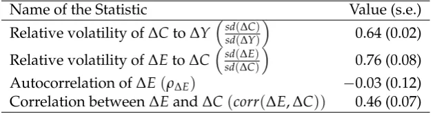
We briefly list the facts we focus on in Table 1. As all variables are measured in changes, we’ll
simply omit “changes” in the remainder of this section.16 First, nondurable consumption is less
12This means nondurables consumption includes both nondurable goods and services.
13We follow Mankiw (1982) to exclude the Korean war period as he argued that the permanent income hypothesis
(PIH) may not hold in that period. Similarly, we also exclude the period surrounding the 2007−2009 Great Recession. For curiosity of readers, we also report statistics using the full sample, i.e., 1955−2012. (See Table 2.)
14Notice that Galí (1993) uses per-capita variables, while we focus on aggregate variables. Using per-capita variables
has little effect on the studied statistics (as many of them are ratios).
15To be consistent with the welfare analysis in Section 4.2 which is based on individual consumption dynamics, we
used per-capita income in the estimation of the income process in the next section. Using aggregate income does not alter the results qualitatively.
volatile than income. The ratio of the standard deviation of nondurable expenditures to the
stan-dard deviation of income is 0.66.17 Second, durable expenditures are less volatile than nondurable
consumption. The ratio of the standard deviation of durable expenditures to the standard
devia-tion of nondurable consumpdevia-tion is 0.62. Third, the autocorreladevia-tion of durable expenditures is−0.3
for the 1955−2007 period. (It is−0.03 for the 1955−2012 period, which is not statistically different
from zero.) Fourth, the correlation between durable expenditures and nondurable consumption is positive but not very large: 0.46.
3. A Stylized Permanent Income Model with Durable Goods
In this section we present a standard full-information rational expectations (FI-RE) version of the permanent income model with durable goods, and discuss the main empirical shortcomings of the model. We will then examine how incorporating slow information diffusion due to noisy signals and slow learning affects the joint behavior of nondurables and durable consumption in the next section. All model economies will be populated by a continuum of infinitely-lived consumers and
prices will be assumed exogenous and constant.18
3.1. The Model
Following Mankiw (1982), Bernanke (1985), and Galí (1993), we consider an FI-RE version of the PIH model which integrates both durable and nondurable consumption, where the latter includes
both nondurable goods and services.19 The optimizing decisions of a representative consumer in
the RE-PIH model with durable goods can be formulated as
max
{ct,kt+1}
(
E0 "∞
∑
t=0
βtu(ct,kt)
#)
, (2)
subject to the budget constraint
at+1= Rat+yt−ct−et, (3)
and the accumulation equation for durables
kt= (1−δ)kt−1+et, (4)
(1982), and Galí (1993).
17As will be clear in later sections, both the standard PIH model and the PIH model with imperfect state observation
implyE[∆C] =E[∆E] =0. We therefore detrend both durable and nondurable consumption data to make the data and the model comparable. Notice that in the PIH model durable and nondurable consumption are not stationary while changes in durable and nondurable consumption are stationary. We also find that using the raw data to compute the key second moments only slightly changes the main results in this paper.
18The benchmark model presented in this paper is usually interpreted as a partial equilibrium PIH model. However,
as noted in Hansen (1987), they can also be interpreted as a general equilibrium model with a linear production tech-nology and an exogenous income process. Specifically, given the expression of optimal consumption derived from the benchmark model, we can price assets by treating optimal consumption as though it were an endowment process. In this setup, equilibrium prices are shadow prices that leave the agent content with that endowment process.
19Although the original Mankiw (1982) model only considers durable consumption, including nondurables
where u(ct,kt) = −21(c−ct)2− ̺2
k−kt
2
is the utility function, c and k are the bliss points,
ct is consumption of nondurables, kt is the stock of durable goods, yt is labor income, et is the
purchase of durable goods,δis the depreciation rate of durable goods, βis the discount factor,R
is the constant gross interest rate, andβR = 1 (an assumption typically imposed in the literature
to guarantee a stochastic steady state).20 Combining (3) and (4) gives the period-to-period finance
constraint of the consumer:
at+1 =Rat+ (1−δ)kt−1−kt+yt−ct. (5)
We define
st =at+ 1−δ
R kt−1+ 1 R
∞
∑
j=0
R−jEtyt+j; (6)
st is the expected present value of lifetime resources, consisting of financial wealth (the risk free
foreign bond), existing stock of durable goods, plus human wealth. Solving this optimization problem gives optimal decisions for nondurable and durable consumption:
ct= Hcst, (7)
kt= R+δ−1
̺ ct =Hkst, (8)
where the marginal propensity to consume out of permanent income,Hc, is
Hc = (R−1) 1+ (1−β(1−δ))
2
β̺
!−1
(9)
andHk = R+̺δ−1Hc(see Appendix 8.1 for derivations).
As shown in Luo (2008), to facilitate the introduction of signal extraction (or rational inatten-tion), we reduce the above multivariate PIH model to a univariate one in which the unique state
variable is permanent incomest that can be solved in closed-form under noisy signals and slow
learning.21 Specifically, ifstis defined as a new state variable, the original finance constraint can
be rewritten as
st+1= Rst−ct−(1−β(1−δ))kt+ζt+1, (10)
where the time(t+1)innovation to permanent income,ζt+1, is
ζt+1= 1
R
∞
∑
j=0
1 R
j
(Et+1−Et)yt+1+j. (11)
20For simplicity, we assume that the price of durable goods in terms of nondurable consumption is 1.
21Reduction of the state space to univariate is particularly convenient for the rational inattention (RI) problem, as
We complete the model description by specifying the income process. Following Quah (1990) and Deaton (1993), we assume that aggregate labor income includes a unit root and the whole income process has two kinds of structural shocks to labor income: One has a permanent impact on the level of labor income and the other has only transitory impact. Specifically, the income process can be written as:
yt+1=ypt+1+yit+1, (12)
ytp+1=ypt +εt+1, (13)
yit+1=y+ǫt+1, (14)
whereytp+1andyit+1are permanent and transitory income components, respectively,εt+1andǫt+1
are orthogonal permanent and transitory iid shocks with mean 0 and varianceω2andω2
ǫ,
respec-tively. As shown in Quah (1990), this two-component income specification provides a potential resolution to Deaton’s puzzle (i.e., the excess smoothness puzzle) in the standard permanent in-come model if the relative importance of transitory to permanent components is large. Here we
estimate the income process using the U.S. data from the period of 1955−2007, and find that
ω2 = 125.72 and ω2
ǫ = 2.42.22 This is consistent with Quah’s (1990) finding that the volatility
of consumption is mainly due to the variations of the permanent component in the income
pro-cess.23 In the permanent income model with durables we presented above, it is straightforward
to show that the income specification can affect the relative volatility of nondurable consumption to income, but has no impact on examining how SID affects the stochastic properties of the joint dynamics of nondurable and durable consumption if consumers can distinguish between the two
components in income.24
In this case, permanent incomest, can be written as
st= at+1−δ
R kt−1+ 1
R−1yt; (15)
that is, st is a linear combination of three state variables, financial wealth, the stock of durable
goods, and labor income. Given the specification of the income process, (12)-(14), the
innova-tion to permanent income can be written as ζt+1 = R−11εt+1+ǫt+1 ∼ N
0,ω2ζ, where ωζ2 =
ω2/(R−1)2+ω2
ǫ ∼= ω2/(R−1)2.25 Combining (7), (8), and (10) gives the expressions for the
22If we use the data set from the 1955−2012 period, and find thatω2 = 131.72 andω2
ǫ = 0.82. The estimation is
implemented using the Matlab toolbox:SSMMATLAB.
23As Tables 1-9 in Quah (1990) show, across different specifications, the variation of the transitory component in the
income process only accounts about 1%−2% of total variation of consumption.
24In Section 4.3, we consider an extension in which consumers cannot distinguish the two components in income. 25Given thatω2=125.72,ω2
changes in nondurable goods and the stock of durable goods:
∆ct = Hcζt, (16)
∆kt = R+δ−1
̺ Hcζt. (17)
(16) is just the random walk result of Hall (1978), and the expenditure on durable goods follows
the ARMA(1, 1)process
et =et−1+ςt−(1−δ)ςt−1, (18)
where ςt = R+̺δ−1
h
1+ (1−β(β̺1−δ))2i−1εt is an unforecastable innovation to consumption at time
t. The MA coefficient is determined entirely by the depreciation rate, δ. In estimating the above
equation using US quarterly data, Mankiw (1982) finds that empirically δ is quite close to 1. In
other words, durables do not look very durable at all and the stochastic behavior of durables purchases seems to be too similar to that of nondurables consumption to be consistent with the
standard PIH’s predictions. Specifically, (18) implies that the first-order autocorrelation of∆etis
ρ∆et ≡corr(∆et,∆et−1) = δ−1
1+ (1−δ)2
<0
because the depreciation rate is less than 1 in the data. For example, if δ = 0.05 (a value that
roughly produces the observed ratio of durables to producer capital in a standard growth model),
ρ∆et = −0.499. However, the estimated value ofρ∆et is far from this number: using the same data
set that Mankiw used, the correlation is 0.06, which implies that the depreciation rate should be 1.07 to make the model fit the data, and more recent data generates similar results (a correlation of
−0.04 impliesδ =0.99527). Tables 1 and 2 report our new estimates ofρ∆etusing the U.S. data from
1955−2007 and 1955−2012, respectively.26 In the two samples, ρ∆et is equal to−0.3 (s.d. 0.07)
and−0.03 (s.d. 0.12), respectively, which requireδ =0.67 andδ =0.97. It is clear that the Mankiw
puzzle still exists. Obviously, a model with this property is going to be difficult to calibrate to observed aggregate data on investment and stocks of durables.
4. Permanent Income Models with Durable Goods and Slow Information Diffusion
In this section, we incorporate slow information diffusion (SID) due to imperfect state observation and slow learning into the otherwise standard permanent income model with durable goods and explore how slow information diffusion due to imperfect observations and slow learning affect the dynamic impacts of income shocks on the joint behavior of nondurables and durables consump-tion.
4.1. Imperfect State Observation and Slow Learning
We assume that consumers in the model economy cannot perfectly observe the true state,
perma-nent income(st), and can only observe a noisy signal
s∗t =st+ξt, (19)
when making decisions, wherestfollows (10) andξtis the iid Gaussian noise due to imperfect
ob-servations. The specification in (19) is standard in the signal extraction (SE) literature and captures the situation where consumers happen or choose to have imperfect knowledge of the
idiosyn-cratic or underlying common shocks.27 It is worth noting that this assumption is also consistent
with the rational inattention (RI) hypothesis proposed by Sims (2003) that ordinary people only devote finite information-processing capacity to processing financial information and thus cannot
observe the states perfectly.28 Although the setting of the original permanent model with durables
presented in the last section is not a typical tracking problem, the filtering problem in this model could be similar to the tracking problem proposed in Sims (2003, 2010). Specifically, we may think that the original model with imperfect state observations can be decomposed into a two-stage op-timization problem:
1. The optimal filtering problem determines the optimal evolution of the perceived (estimated) state;
2. The optimal control problem in which the decision makers treat the perceived state as the
underlying state when making optimal decisions.29
Since the filtering problem here can be considered as a standard tracking problem, we know from Sims (2003) and Makowiak and Wierderholt (2009) that the optimal RI-induced noise is an iid Gaussian variable. It is worth noting that in the traditional SE problem, we do not have such restriction on the stochastic properties of the noises, and the fundamental variable could be
corre-lated with the exogenous noise.30 In this paper, we focus on the iid noise case as it can be
rational-ized by the RI theory.
Since imperfect observations on the state lead to welfare losses, households use the processed
information to estimate the true state.31 Specifically, we assume that households use the Kalman
filter to update the perceived statebst = Et[st] after observing new signals in the steady state in
which the conditional variance ofst,Σt=vart(st), has converged to a constantΣ:
bst+1= (1−θ) [Rbst−ct−(1−β(1−δ))kt] +θs∗t+1 (20)
27For example, Muth (1960), Lucas (1972), Lorenzoni (2009), and Angeletos and La’O (2010, 2012).
28As shown by Shannon (1948), measuring a real-value stochastic process without error implies an infinite amount of
information-processing capacity.
29See Liptser and Shiryayev (1991) for a textbook treatment on this topic and an application in a precautionary saving
model in Wang (2004).
30See Luo and Young (2014) for a discussion on this issue.
whereθis the Kalman gain (i.e., the optimal weight on any new observation).32 In the signal extraction problem, the Kalman gain can be written as
θ=ΣΛ−1, (21)
where Σ is the steady state value of the conditional variance of st+1, vart+1(st+1), and Λ =
vart(ξt+1)is the variance of the noise. Σ and Λare linked by the following updating equation
for the conditional variance in the steady state:
Λ−1 =Σ−1−Ψ−1, (22)
where Ψ is the steady state value of the ex ante conditional variance of st+1, Ψt = vart(st+1).
Multiplyingω2
ζ (the variance of the innovation tos) on both sides of (22) and using the fact that
Ψ= R2Σ+ωζ2, we have
ωζ2Λ−1 =ω2ζΣ−1−
R2ω2ζΣ−1−1+1
−1
, (23)
whereωζ2Σ−1=ω2
ζΛ−1
ΛΣ−1.
Define the signal-to-noise ratio (SNR) asπ= ω2
ζΛ−1. We obtain the following equality linking
πand the Kalman gain(θ):
π= θ
1
1−θ −R
2
. (24)
Solving forθyields
θ = −(1+π) +
q
(1+π)2+4R2(π+R2)
2R2 , (25)
where we omit the negative values ofθbecause bothΣandΛmust be positive. It is straightforward
to show thatθandπhave one-to-one monotonic relationship. Note that givenπ, we can pin down
Λusingπ =ωζ2Λ−1andΣusing (21) and (25).
Notice that this signal extraction problem with exogenously specified noises is observation-ally equivalent to the RI model with endogenous noises and fixed (or elastic) capacity. Specifi-cally, consumers under RI face both the usual flow budget constraint as well as an information-processing constraint due to finite Shannon capacity. Following Sims (2003), the typical con-sumer’s information-processing constraint can be characterized by the inequality
H(st+1|It)− H(st+1|It+1)≤κ, (26)
whereIt is the consumer’s currently processed information, κ is the consumer’s channel
capac-ity, H(st+1|It) denotes the entropy of the state prior to observing the new signal at t+1, and
32Note thatθmeasures how much uncertainty about the state can be removed upon receiving the new signals about
H(st+1|It+1)is the entropy after observing the new signal. (26) implies that the reduction in the
uncertainty about the state variable gained from observing a new signal is bounded by κ. As
shown in Sims (2003), within the linear-quadratic-Gaussian setting, Dt is a normal distribution
N(bst,Σt); as a result, (26) can be reduced to
ln|Ψt| −ln|Σt+1|=2κ (27)
whereΣt+1 = var(st+1| It+1)andΨt = var(st+1| It)are the posterior and prior variances of the
state variable, respectively. In this univariate case, (27) has the steady stateΣ= ω2ζ
exp(2k)−R2, and the
consumer behaves as if observing a noisy measurement of permanent incomes∗t+1 = st+1+ξt+1,
whereξt+1 is the endogenous noise with mean 0 and variance Λt = var(ξt+1| It); in the steady
stateΛ= Σ−1−Ψ−1−1and the Kalman gain:
θ =ΣΛ−1=1− 1
exp(2κ), (28)
is the optimal weight on any new observation. Comparing (25) with (28), it is clear that if the SNR and capacity satisfy
π =
1− 1
exp(2κ)
exp(2κ)−R2, (29)
the SE and RI problems are observationally equivalent in the sense that they lead to the same
model dynamics governed byθ. (29) clearly shows that the SNR is an increasing function of
chan-nel capacity. In addition, as argued in Sims (2010), instead of assuming that chanchan-nel capacity is fixed, it is also reasonable to assume that the marginal cost of information processing is constant such that capacity can be elastic in response to a change in environment. In other words, the
La-grange multiplier on (27),λ, is constant. As these two modeling strategies are also observationally
equivalent in the sense that they lead to the same model dynamics, here we just use the Kalman
gainθto characterize the degree of SID.33
4.2. Individual Dynamics and Welfare Implications under SID
Combining (19) with (20), we obtain the following proposition about the dynamic behavior of the
perceived statebst:
Proposition 1. Under SID,bstfollows:
b
st+1 =Rbst−ct−(1−β(1−δ))kt+ηt+1, (30)
where
ηt+1 =θ
ζt+1
1−(1−θ)R·L
+
ξt+1− θRξt
1−(1−θ)R·L
, (31)
ω2ξ =var(ξt+1) = 1
θ
1
1/(1−θ)−R2ω
2 ζ,
ω2η =var(ηt+1) = θ
1−(1−θ)R2ω
2
ζ >ωζ2, forθ <1, (32)
and we use the fact that the estimation error, st−bst, can be written as
st−bst= (1−θ)ζt
1−(1−θ)R·L −
θξt
1−(1−θ)R·L. (33)
Expression (33) shows that the estimation error reacts to the fundamental shock positively, while it reacts to the noise shock negatively. In addition, the importance of the estimation error is
decreasing withθ. More specifically, asθ increases, the first term in (33) becomes less important
because(1−θ)ζt in the numerator decreases, and the second term also becomes less important
because the variance ofξtdecreases asθincreases.
The optimization problem for the typical household facing state uncertainty can thus be refor-mulated as
v(bst) = max
{ct,kt}{Et[u(ct,kt) +βv(bst+1)]} (34)
subject to (30)-(32), and givenbs0. Solving this Bellman equation yields the following proposition:
Proposition 2. Under SID, the consumption and durable accumulation functions are
ct= Hcbst (35)
kt= Hkbst, (36)
where Hcis defined in (9) and Hk = 1−ββ̺(1−δ)Hc, and the value function is
v(bst) = A0+A1bst+A2bs2t, (37)
where A2 =−R(2R−Θ1), A1= Rc, and A0=−2(RR−Θ1)c2− 2RΘvar(ηt+1).
Proof. See Appendix 8.3.
Whenθ = 1, i.e., in the FI-RE case, the consumption functions reduce to (35) and (36),
respec-tively, and the value function reduces to
e
v(st) = A0+A1st+A2s2t,
imperfect-state-observation cannot help in individuals’ optimization – consumers with finite capacity cannot ob-serve the state perfectly when making optimal decisions – the average welfare difference between the RI and FI-RE economies is greater than 0. We examine here the welfare cost of RI – how much utility does a consumer lose if the actual consumption path he chooses under SID deviates from the first-best FI-RE path? Specifically, following Barro (2007) and Luo and Young (2010), given the
initial value of the state,bs0, the marginal welfare costs (mwc) due to SID in our benchmark model
can be written as
mwc≡ −(∂v∂v((bs0)/∂θ
bs0)/∂bs0)bs0
=− 1
2[(R−1)bs0−Θc]bs0
∂ω2η
∂θ
This expression gives the proportionate reduction in the initial level of the perceived state(bs0)that
compensates, at the margin, for a decrease inθ (i.e., stronger SID) — in the sense of preserving
the same effect on welfare for a givenbs0. To do quantitative welfare analysis we need to know the
levels ofbs0 andc. First, denote by γ the local coefficient of relative risk aversion, which equals
γ = c−EE[y[]y] for the utility functionu(·)evaluated at mean incomeE[y]. Using the U.S. data from
the 1955−2007 period, we haveE[yt] =16798,ω =125.7 , andωǫ=2.4 (all in 2005 U.S. dollars),
and then find the value of the bliss pointcthat generates reasonable relative risk aversionγ. For
example, ifγis equal to 1.5,c = 1.5E[yt]. Furthermore, assume that the ratio of the initial level
of financial wealth(ba0)to mean income (yb0 ≡E[yt])is 5, that is, ba0/yb0 = 5.34 Given thatbs0 =
b
a0+ 1−Rδbk0+ R1−1yb0, we can calculate that mwc = 9. 89×10−4 whenθ = 0.5, using the fact that
∂ω2 η
∂θ = 1−R
2
[1−(1−θ)R2]2ω
2
ζ < 0. Therefore, to maintain the level of the value function, an increase in
θ of 100 percent (from 0.5 to 1) requires a reduction in the initial level of bs0 by approximately
0.049 percent.35 This result thus provides some evidence that it is reasonable for consumers to
learn the true state slowly due to finite capacity because the welfare improvement from increasing learning capacity is trivial. In other words, although consumers can devote much more capacity to processing economic information and then improve their optimal consumption decisions, it is rational for them not to do so because the welfare improvement is tiny. This result is consistent with that obtained in the models without durable consumption, e.g., Pischke (1995) and Luo and Young (2010).
Using (35) and (36), straightforward calculations imply that
∆ct =θHc
ζt
1−(1−θ)R·L +
ξt− θRξt−1
1−(1−θ)R·L
, (38)
∆kt =θHk
ζt
1−(1−θ)R·L+
ξt− θRξt−1
1−(1−θ)R·L
, (39)
34This number varies largely for different individuals, from 2 to 20. 5 is the average wealth/income ratio in the
Survey of Consumer Finances 2001. We find that changing the value of this ratio only has minor effects on the welfare implication.
35This result is robust to the change in the value ofθ. For example, whenθ=0.6,mwc=6.775×10⁻⁴, and an increase
inθby 66.7 percent (from 0.6 to 1) requires a reduction in the initial level ofbs0by approximately 0.027 percent in order
where we use the fact that∆bst = θh ζt
1−(1−θ)R·L+
ξt−1−θ(1R−ξtθ−)1R·L
i
. Hence, under the innocuous
assumption that(1−θ)R <1, both consumption processes follow MA(∞)processes.36
Expendi-ture on durable goods follows the process
∆et =θHk
ζt+ ((1−1θ−)R(1−−(1θ−)R·Lδ))ζt−1
+
ξt−(1−δ+θR)ξt−1+θR((1−1−δ)(−1−(1θ−)RLθ)R)ξt−2
, (40)
which reduces to∆et =Hkζtwhenθ=1.
4.3. Aggregation
Our model economy is now populated by a continuum of ex ante identical but ex post heteroge-neous consumers because consumers face the idiosyncratic noise shock. Sun (2006) presents an law of large numbers for this type of economic models and then characterizes the cancellation of indi-vidual risk via aggregation. In this paper, following Uhlig (1996) and Zaffaroni (2004), we show that the idiosyncratic RI-induced noises can be exactly cancelled out after aggregating across all
agents if they converge in mean square to the population mean(0). Specifically, after aggregating
over all consumers under an assumption of identicalθ, we obtain the expressions for changes in
aggregate nondurables and durables:
∆Ct =θHc
ζt
1−(1−θ)R·L
, (41)
∆Kt = 1−β(1−δ)
β̺ ∆Ct, (42)
and
∆Et= θHk
ζt+
((1−θ)R−(1−δ))ζt−1
1−(1−θ)R·L
, (43)
respectively (see Appendix 8.4 for the proof). It is worth noting that the assumption of convergence in mean square helps resolve the impossibility result discussed in Judd (1985) and Feldman and
Gilles (1985).37
Equations (41)-(43) clearly show that SID can help generate the smooth and hump-shaped im-pulse responses of nondurables and durables consumption to the income shock. More specifically, we explore how SID affects the stochastic properties of the joint dynamics of income, nondurables, and durables along the following key dimensions: (i) the relative volatility of nondurables to in-come, (ii) the relative volatility of expenditures on durables and nondurables, (iii) the first-order autocorrelation of changes in durables expenditures, and (iv) the contemporaneous correlation be-tween nondurables and durable expenditures. After inspecting the third aspect above, we easily
36This assumption only has bite whenθis very close to 0 where the absence of precautionary motives due to quadratic
utility is likely to be problematic.
37The impossibility result says that if agents in a continuum population face idiosyncratic uncertainty, the strong law
determine whether the Mankiw puzzle can be resolved by breaking the tight link between the MA coefficient and the depreciation rate implied by the FI-RE assumption.
5. Empirical Implications
5.1. Stochastic Properties of Nondurable and Durable Consumption
5.1.1. The Relative Volatility of∆Ctto∆Yt
Given (41) and (43), the relative volatility of the changes in nondurable consumption to income can be written as:
µ≡ sd(∆Ct)
sd(∆Yt)
= 1+ (1−β(1−δ))
2
β̺
!−1s
θ2
1−((1−θ)R)2, (44)
whereΘ≡
r θ2
1−((1−θ)R)2.
Proposition 3.
∂µ
∂θ >0. (45)
Proof. It’s straightforward to show ∂∂θΘ >0. Thus,∂µ ∂θ >0.
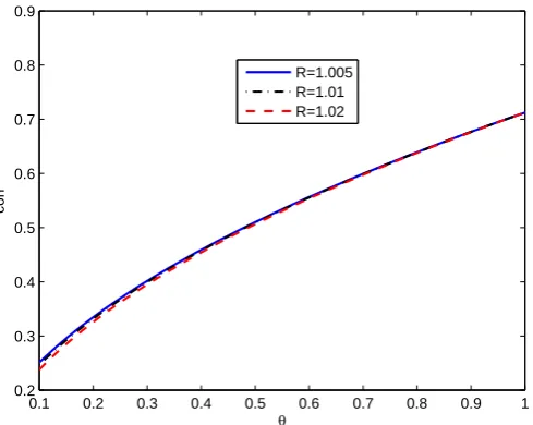
The above proof shows that slow learning reduces the relative volatility µ via an additional
factor due to SID,Θ. Figure 1 illustrates howθ affectsΘ. It clearly shows that slow learning due
to noisy state observations increases the excess smoothness of nondurables relative to income. As
shown in Table 3, whenθ =0.62, i.e., 62 percent of any new information is transmitted each period
(equivalently 62 percent of the uncertainty is removed upon the receipt of a new signal),µ=0.66,
exactly what it is in the data. It is not difficult to understand why SID reduces the relative volatility
of nondurable consumption. As (41) shows, the nondurable consumption changes,∆Ct, becomes
an MA(∞) process, meaning that it not only depends on the current innovation but also is
in-fluenced by innovations in previous periods. This makes nondurable consumption change more gradually, and therefore has a lower volatility. In addition, as well documented in the consump-tion literature (e.g., Deaton (1992) and Reis (2006)), the impulse response of aggregate nondurable consumption to aggregate income takes a hump-shaped form, which means that aggregate con-sumption reacts to income shocks gradually and with delay.
5.1.2. The Relative Volatility of∆Etto∆Ct
Given (41) and (43), the relative volatility of the changes in durable to nondurable consumption can be defined as follows
rv≡ sdsd((∆∆CEt)
t)
=
R+δ−1
̺
q
where sd(∆Ct)and sd(∆Et)are standard deviation of∆Ctand∆Et, respectively.
Proposition 4.
∂(rv)
∂θ >0.
Proof. This can easily be proved by simply illustrating that the second term on the right-hand side
of (46) monotonically increases with the degree of slow learning,θ.
This proposition is very interesting and probably requires more explanations. First of all, it says that changes in durable consumption become less volatile than changes in nondurable
consump-tion under SID.38Given that Proposition 3 shows that SID can reduce the volatility of nondurable
consumption changes, it is not surprising to see that it can also reduce the volatility of durable consumption changes. The question is why SID reduces the volatility of durable consumption changes more than that of nondurable consumption changes. The key reason that the change in
durable consumption is actually more volatile than that in the stock of durables whenδ<1 is due
to the MA representation of∆Et. (Note that in this case, 1+ (1−δ)2 > 1, and SID measured by
θ<1 smooths the process for the stock of durables and nondurables in a similar fashion as shown
by (41) and (43).) In other words, the depreciation channel(δ<1)in this case has the potential to
increase the relative volatility of∆Etto∆Ct. When the depreciation rate is 100 percent, theCtand
Kt processes are essentially the same and thus SID has no impact on the relative volatility of the
change in durable consumption to that in nondurable consumption. In contrast, in the presence of
SID, i.e.,θ <1, (41) and (43) clearly show that the SID channel offsets the depreciation channel and
thus reduces the relative volatility of∆Etto∆Ct.39
Second, it is worth noting thatE[∆Ct] = E[∆Kt] =0 in the model with SID.40This means that
the variations of∆Ctand∆Kt+1 are not influenced by their levels (as both are zero, on average).
Therefore, it excludes the possibility that SID reduces sd(∆Ct)/ sd(∆Et)by altering the relative
size of∆Cto∆E.
Another way to examine how SID affects the relative variability is to define
Π≡ rv(θ =1)
rv(θ <1) =
v u u
t 1+ (1−δ)2
1+ (1−δ)2−2(1−δ) (1−θ)R. (47)
Figure 2 clearly shows that the presence of SID governed byθcan improve the model’s prediction
for the observed variability ratio for different values of R. An example is when δ = 0.05 and
θ = 0.1,Π = 3.7, that is, if 10 percent of the uncertainty is removed upon the receipt of a new
signal, the predicted relative variability can be reduced by about 4 times.
38As Table 4 shows, the standard FI-RE model predicts a relative volatility of durable to nondurable larger than 1.
Similar evidence has been documented in Galí (1993) as well.
39Note that in the expression for∆E
t, the 1−(1−θ)R·Lterm makes the process smoother and(1−θ)R−(1−δ)
also reduces the initial impact of the depreciation channel.
5.1.3. The First-order Autocorrelation of∆Et
By construction, (43) can be rewritten as
∆Et =ςt+
((1−θ)R−(1−δ))ςt−1
1−(1−θ)R·L , (48)
whereςt = R+̺δ−1θHcζt with var(ςt) =
R+δ−1 ̺ θHc
2
ω2
ζ. Given (48), the first-order
autocorrela-tion of∆Etcan be written as follows:
ρ ≡ cov(∆Et+1,∆Et)
var(∆Et)
= (1−θ)R−(1−δ) 1−((1−θ)R)
2
1+ (1−δ)2−2(1−δ) (1−θ)R. (49)
Based on (49), the following proposition shows how the combination of(θ,δ)affects the first-order
autocorrelation of the expenditure on durables.41
Proposition 5.
∂ρ ∂θ <0,
∂ρ ∂δ >0.
Proof. Given (49), it is straightforward to show that ∂ρ∂θ <0 becauseθ,(1−θ)R∈(0, 1), and
∂ρ ∂δ =
1−(1−δ)2 h1−((1−θ)R)2i
h
1+ (1−δ)2−2(1−δ) (1−θ)Ri2
>0.
This proposition shows that SID increases the first-order autocorrelation of∆Et, i.e., the less the
value ofθ, the largerρ. Figure 3 illustrates howρincreases with the degree of SID. In addition, the
higher the depreciation rate, the largerρ. For example, givenR=1.01 andδ =0.05,ρ=0.5 when
θ = 1,ρ = −0.25 whenθ = 0.5, andρ = −0.03 whenθ =0.1. These results suggest that SID has
the potential to resolve the Mankiw puzzle.
5.1.4. The Correlation between∆Etand∆Ct
Given (41) and (43), the contemporaneous correlation between the changes in durable and non-durable consumption can be written as:
corr(∆Et,∆Ct)≡ cov(∆Et,∆Ct)
sd(∆Ct)sd(∆Et) =
1−(1−δ) (1−θ)R
q
1+ (1−δ)2−2(1−δ) (1−θ)R
, (50)
We then have the next result.
Proposition 6.
∂corr(∆Et,∆Ct)
∂θ >0. (51)
Proof. The proof is straightforward.
Here is some intuition on why SID reduces the contemporaneous correlation between the changes in nondurable and durable consumption. From Proposition 4 we see that SID reduces relative volatility of durable consumption changes to nondurable consumption changes, meaning that SID makes durable consumption respond more gradually to income shocks than nondurable consumption. Figure 4 illustrates how the contemporaneous correlation between durable and
non-durable consumption decreases with the degree of SID (i.e., lessθ). Intuitively, as durable
con-sumption and nondurable concon-sumption respond to income shocks in increasingly different ways, the correlation between them also declines.
5.2. Quantitative Results
The previous section provides qualitative results based on the closed-form solutions which show that introducing SID can help a standard PIH model with both durable and nondurable goods better explain the four dimensions of durable and nondurable consumption. In particular, Propo-sitions 3-6 have shown that all these improvements are driven by the change of one single
param-eter,θ, which is the optimal weight on any new observation (or the Kalman gain). That is, based
on a standard framework used in the literature, our analysis highlights the effects of information frictions on the model implications for the joint dynamics of durable and nondurable consumption.
This section quantifies the improvement in model predictions through assigning values for this
key parameter,θ. Generally speaking, there are multiple ways we can choose a value forθ. For
instance, we can set different values forθ to match each of the four dimensions we studied in the
previous section. However, as the focus of this analysis is on how SID helps explain the behavior
of durable goods, we will not use the moments involving durable consumption to calibrateθ. So,
in the calibration,θis chosen to match the observed relative volatility of nondurable consumption
to income in the data.42
Before going to the results, Table 3 reports the values for other parameters used to generate the quantitative results. In choosing values for these parameters, we closely follow the literature,
which allows us to focus on the effects of our key SID parameter(θ)on changing the model
pre-dictions. The preference parameter̺is chosen from Bernanke (1985). The (quarterly) depreciation
rate for durable goods is set to be 1.5 percent which lies well in the range used in the literature.
42Estimatingθwithout using a model is difficult; estimates in the literature exist for the amount of information that
For example, Bernanke (1985) uses 2.5 percent and Monacelli (2009) uses 1 percent (i.e., annually 4 percent).
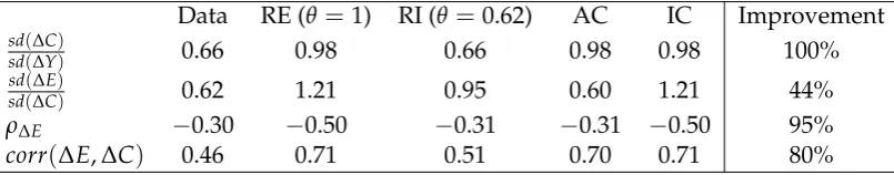
Table 4 reports the quantitative results using data from the period 1955−2007 and the results
for the period 1955−2012 are reported in Table 5. These tables clearly show that SID can
sig-nificantly improve the model’s quantitative predictions on the joint dynamics of nondurable and
durable consumption. Particularly, the main conclusion from these results is that a value of θ
which matches the relative volatility of nondurable consumption to income significantly improves the model predictions along the other three dimensions of durable consumption as well.
Specif-ically, using the 1955−2007 data, whenθ = 62 percent, the SID model can improve the model’s
prediction on the relative volatility of durable to nondurable consumption, the first-order auto-correlation of durable consumption, and the contemporaneous auto-correlation between durable and
nondurable consumption by 44 percent, 95 percent, and 80 percent, respectively.43 As a reminder,
we are not directly choosingθto match any moments on durable consumption (although this can
easily be done). Thus, these results suggest that the SID mechanism is important for explaining the behavior of durable consumption.
6. Extensions and Discussion
6.1. Bernanke’s Adjustment Costs (AC) Model
The main difference between the model present in Section 3.1 and the model in Bernanke (1985) is that the latter assumes changing durables stocks involves quadratic adjustment costs because pur-chases of durables require leisure expenditure. Specifically, the utility function of a representative
consumer during a given periodtis assumed to be
u(ct,kt,kt−1) =−1
2(c−ct)
2
− ̺
2
k−kt
2
− ϑ
2 (kt−kt−1)
2, (52)
whereϑ measures the importance of adjustment costs in utility.44 Solving this model yields the
following dynamics for nondurable and durable consumption:
∆ct= GcGyεt, (53)
∆kt= x1(1−β(1−δ))
ϑ1−x−21
GcGyεt
1−x1·L, (54)
whereLis the lag operator. (See Appendix 8.5 for the derivation.)
Clearly, (54) is an MA(∞)process with decreasing MA coefficients, which means that durables
43Using the 1955−2012 data andθ=60%, we find that SID can improve these three dimensions by 62%, 43%, and
80%, respectively.
44Bernanke (1985) assumes that utility is a non-separable function of nondurables and durables consumption; that
is, there is an additional term−m(c−ct)
k−kt
consumption reacts to the income shock gradually in the presence of adjustment costs. Figure 1
illustrates the impulse responses of durables consumption growth∆kt to the income shock when
the parameters are the same as that estimated in Bernanke (1985) (R =1.01,ϑ= 0.706,δ =0.025,
̺ = 0.0286, x1 = 0.828). Expression (54) also shows that the presence of adjustment costs can
improve the model’s predictions in the following aspects: (1) it increases excess smoothness of durables consumption and (2) it increases the autocorrelation of durables consumption by intro-ducing a slow adjustment mechanism.
However, although the presence of adjustment costs reduces the initial response of nondurables
consumption to the income shock because GcGy < 1 when ϑ > 0 as is clear in Equation (53),
it does not affect the dynamic responses of nondurables consumption, which is still the random
walk result of Hall (1978).45 Specifically, the introduction of adjustment costs reduces the relative
volatility of aggregate nondurables consumption to income, defined as
µ= sd(∆Ct)
sd(∆Yt) =
1+ (1−β(1−δ))2 R
R−x1
x1
ϑ1−x−21
−1
<1.
Using the same parameter values as in the last section, we find thatµ=0.98, which is the same as
that obtained in the FI-RE model and is well above its empirical counterpart(0.66). In other words,
costs of adjusting durable stocks do not improve the model’s predictions for the joint behavior of aggregate nondurables consumption and income sufficiently; in US data nondurables consump-tion is much smoother than income. In addiconsump-tion, it is clear from (53) that the impulse response of aggregate nondurable consumption to aggregate income is flat with an immediate upward jump in the initial period that persists indefinitely, which is not consistent with the VAR evidence docu-mented in the literature that the impulse response of aggregate nondurable consumption to income takes a hump-shaped form.
To compare the AC model with the SID model, we setx1= (1−θ)Rsuch that the two models
have the same propagation mechanism in the dynamics of durable consumption. We report the results in Tables 4-5. It is clear from the tables that SID did a better job in explaining the relative volatility of nondurable consumption to income and the contemporaneous correlation between nondurable and durable consumption: The AC model’s predictions on these two moments are the same as that obtained in the FI-RE model. It is worth noting that the AC model’s prediction on the relative volatility of durable to nondurable consumption matches the data better than the SID model at the cost of worsening the model’s prediction on the relative volatility of nondurable
consumption to income.46
45In other words, nondurable consumption is not sensitive to past information, as predicted by the standard
perma-nent income model.
46Note thatsd(∆E)
sd(∆C) =
sd(∆E)
sd(∆Y)/
sd(∆C)
6.2. Incomplete Information about Current Income (IC)
In this subsection, we consider an extended incomplete information (IC) model in which con-sumers cannot distinguish the two components in income specified in (12)-(14). Specifically, fol-lowing Muth (1960) and Pischke (1991), given that the change in income is
∆yt+1=εt+1+ǫt+1−ǫt, (55)
the best forecast is to recognize that∆yt+1is a moving-average process of order one:
∆yt+1=νt+1−ανt, (56)
where the innovation,νt, with mean 0 and varianceων2, is not a fundamental driving process – it
contains information on current and lagged permanent and transitory income shocks. Equating the variances and autocorrelation coefficients of the original and derived processes (55) and (56), we have
ω2ν =
ω2ǫ
α , α=−1−
p
1−4̺2
2̺ ,
where̺ = − ωǫ2
ω2+2ω2
ǫ andα ∈ [0, 1]will be large if the variance of the transitory shockω
2
ǫ is large
relative to the variance of the permanent shockω2and will converge to 0 asω2ǫapproaches to 0.
Following the same procedure in Section 4.1, the new state variable and the original budget constraint can be written as:
st =at+ 1−δ
R kt−1+ 1 R−1y
p t −
α
R−1νt, st+1 =Rst−ct−(1−β(1−δ))kt+ζt+1,
respectively, whereζt+1 = R−R−α1νt+1. The expressions for changes in aggregate nondurables and
durables can then be rewritten as:
∆Ct =Hc R−α
R(R−1)
θεt+1
(1−(1−θ)R·L) (1−α·L)
, (57)
∆Kt = 1−β(1−δ)
β̺ ∆Ct. (58)
respectively, where the iid idiosyncratic noises in the expressions for individual consumption dy-namics are canceled out. These equations bring out two salient points in our extended model. First, both SID and incomplete information provide endogenous propagation mechanisms of the
model – they are characterized by the two factors, 1−(1−1θ)R·L and 1−1α·L, respectively, and thus