Munich Personal RePEc Archive
Analogy Making and the Structure of
Implied Volatility Skew
Siddiqi, Hammad
1 October 2014
1
Analogy Making and the Structure of Implied Volatility Skew
1Hammad Siddiqi
University of Queensland
[email protected] This version: December 2014.
An analogy based call option pricing model is put forward. The model provides a new explanation for the implied volatility skew puzzle and is consistent with empirical findings regarding leverage adjusted option returns. It explains puzzling superior performance of covered call writing and worse-than-expected performance of zero-beta straddles. The analogy based stochastic volatility and the analogy jump diffusion models are also developed. The analogy based stochastic volatility model generates the skew even without any correlation between the stock price and volatility processes, whereas, the analogy jump diffusion does not require asymmetric jumps to generate the skew.
JEL Classification: G13, G12
Keywords: Implied Volatility Skew, Implied Volatility Smile, Stochastic Volatility, Jump Diffusion, Covered Call Writing, Zero-Beta Straddle, Leverage Adjusted Option Returns
1
2
Analogy Making and the Structure of Implied Volatility Skew
The existence of the implied volatility skew is perhaps one of the most intriguing anomalies in
option markets. According to the Black-Scholes model (Black and Scholes (1973)), volatility inferred
from prices (implied volatility) should not vary across strikes. In practice, a sharp skew in which
implied volatilities fall monotonically as the ratio of strike to spot increases is observed in index
options.
The Black-Scholes model assumes that an option can be perfectly replicated by a portfolio
consisting of continuously adjusted proportions of the underlying stock and a risk-free asset. The
cost of setting up this portfolio should equal the price of the option. Most attempts to explain the
skew have naturally relaxed the assumption of perfect replication. Such relaxations have taken two
broad directions: 1) Deterministic volatility models 2) Stochastic volatility models without jumps and
stochastic volatility models with jumps. In the first category are the constant elasticity of variance
model examined in Emanuel and Macbeth (1982), the implied binomial tree models of Dupire
(1994), Derman and Kani (1994), and Rubinstein (1994). Dumas, Fleming and Whaley (1998)
provide evidence that deterministic volatility models do not adequately explain the structure of
implied volatility as they lead to parameters which are highly unstable through time. The second
broad category is examined in papers by Chernov et al (2003), Anderson, Benzoni, and Lund (2002),
Bakshi, Cao, and Chen (1997), Heston (1993), Stein and Stein (1991), and Hull and White (1987)
among others. Bates (2000) presents empirical evidence regarding stochastic volatility models with
and without jumps and finds that inclusion of jumps in a stochastic volatility model does improve
the model, however, in order to adequately explain the skew, unreasonable parameter values are
required. Generally, stochastic volatility models require an unreasonably strong and fluctuating
correlation between the stock price and the volatility processes in order to fit the skew, whereas,
jump diffusion models need unreasonably frequent and large asymmetric jumps. Empirical findings
suggest that models with both stochastic volatility and jumps in returns fail to fully capture the
empirical features of index returns and option prices (see Bakshi, Cao, and Chen (1997), Bates
(2000), and Pan (2002)).
Highly relevant to the option pricing literature is the intriguing finding in Jackwerth (2000)
3 investor. Perhaps, another line of inquiry is to acknowledge the importance of heterogeneous
expectations and the impact of resulting demand pressures on option prices. Bollen and Whaley
(2004) find that changes in implied volatility are directly related to net buying pressures from public
order flows. According to this view, different demands and supplies of different option series affect
the skew. Lakonishok, Lee, Pearson, and Poteshman (2007) examine option market activity of
several classes of investors in detail and highlight the salient features of option market activity. They
find that a large percentage of calls are written as a part of covered call strategy. Covered call writing
is a strategy in which a long position in the underlying stock is combined with a call writing position.
This strategy is typically employed when one is expecting slow growth in the price of the underlying
stock. It seems that call buyers expect higher returns from the underlying stock than call writers, but
call writers are not pessimistic either. They expect slow/moderate growth and not a sharp downturn
in the price of the underlying stock.
Should expectations regarding the underlying stock matter for option pricing? In the
Black-Scholes world where perfect replication is assumed, expectations do not matter as they do not affect
the construction of the replicating portfolio or its dynamics. However, empirical evidence suggests
that they do matter. Duan and Wei (2009) find that a variable closely related to the expected return
on the underlying stock, its systematic risk proportion, is priced in individual equity options.
There is also strong experimental and other field evidence showing that the expected return
on the underlying stock matters for call option pricing. Rockenbach (2004), Siddiqi (2012), and
Siddiqi (2011) find that participants in laboratory experiments seem to value a call option by
equating its expected return to the expected return available from the underlying stock. From this
point onwards, we refer to this as the analogy model. In the field, many experienced option traders
and analysts consider a call option to be a surrogate for the underlying stock because of the
similarity in their respective payoffs.2 It seems natural to expect that such analogy making/similarity
argument influences option valuation, especially when it comes from experienced market
professionals. Furthermore, as a call option is defined over some underlying stock, the return on the
underlying stock forms a natural benchmark for forming expectations about the option. This article
puts forward an analogy based call option pricing model and shows that it provides a new
2 As illustrative examples, see the following:
http://ezinearticles.com/?Call-Options-As-an-Alternative-to-Buying-the-Underlying-Security&id=4274772, http://www.investingblog.org/archives/194/deep-in-the-money-options/, http://www.triplescreenmethod.com/TradersCorner/TC052705.asp,
4 explanation for the implied volatility skew puzzle. The analogy model is also shown to be consistent
with recent empirical findings regarding leverage adjusted option returns (Constantinides et al
(2013)). The model also explains the superior performance of covered call writing and
worse-than-expected performance of zero-beta straddles.
In a laboratory experiment, it is possible to objectively fix the expected return available on
the underlying stock and make it common knowledge, however, in the real world; people are likely
to have different subjective assessments of the expected return on the underlying stock. An analogy
maker expects a return from a call option which is equal to his subjective assessment of the expected
return available on the underlying stock. The marginal investor in a call option is perhaps more
optimistic than the marginal investor in the corresponding underlying stock. To see this, consider
the following: In the market for the underlying stock, both the optimistic and pessimistic beliefs
influence the belief of the marginal investor. Optimistic investors influence through demand
pressure, whereas the pessimistic investors constitute the suppliers who influence through selling
and short-selling. However, highly optimistic investors should favor a call option over its underlying
stock due to the leverage embedded in the option. Furthermore, in the market for a call option,
covered call writers are typical suppliers (see Lakonishok et al (2007)). Covered call writers are
neutral to moderately bullish (and not pessimistic) on the underlying stock. Hence, due to the
presence of relatively more optimistic buyers and sellers, the marginal investor in a call option is
likely to be more optimistic about the underlying stock than the marginal investor in the underlying
stock itself. Hence, the expected return reflected in a call option is likely to be larger than the
expected return on the underlying stock. Also, as more optimistic buyers are likely to self-select into
higher strike calls, the expected return may rise with strike.
If analogy makers influence call prices, shouldn’t a rational arbitrageur make money at their expense by taking an appropriate position in the call option and the corresponding replicating
portfolio in accordance with the Black Scholes model? Such arbitraging is difficult if not impossible
in the presence of transaction costs. In continuous time, no matter how small the transaction costs
are, the total transaction cost of successful replication grows without bound rendering the
Black-Scholes argument toothless. It is well known that there is no non-trivial portfolio that replicates a
call option in the presence of transaction costs in continuous time. See Soner, Shreve, and Cvitanic
(1995). In discrete time, transaction costs are bounded, however, a no-arbitrage interval is created. If
5 conditions under which this happens in a binomial setting. Of course, if the underlying stock
dynamics exhibit stochastic volatility or jump diffusion then the Black-Scholes argument does not
hold irrespective of transaction costs and/or other limits to arbitrage. Hence, analogy makers cannot
be arbitraged away in that case.
Analogy making is complementary to the approaches developed earlier such as stochastic
volatility and jump diffusion models. Such models specify certain dynamics for the underlying stock.
The idea of analogy making is not wedded to a particular set of assumptions regarding the price and
volatility processes of the underlying stock. It can be applied to a wide variety of settings. In this
article, first we use the setting of a geometric Brownian motion. Then, we integrate analogy making
with jump diffusion and stochastic volatility approaches. Combining analogy making and stochastic
volatility leads to the skew even when there is zero correlation between the stock price and volatility
processes, and combining analogy making with jump diffusion generates the skew without the need
for asymmetric jumps.
This article is organized as follows. Section 1 summarizes existing evidence pointing to
analogy based call option pricing. Section 2 builds intuition by providing a numerical illustration of
call option pricing with analogy making. Section 3 develops the idea in the context of a one period
binomial model. Section 4 puts forward the analogy based option pricing formulas in continuous
time. Section 5 shows that if analogy making determines option prices, and the Black-Scholes model
is used to back-out implied volatility, the skew arises, which flattens as time to expiry increases.
Section 6 shows that the analogy model is consistent with key empirical findings regarding returns
from covered call writing and zero-beta straddles. Section 7 shows that the analogy model is
consistent with empirical findings regarding leverage adjusted option returns. Section 8 puts forward
an analogy based option pricing model when the underlying stock returns exhibit stochastic
volatility. It integrates analogy making with the stochastic volatility model developed in Hull and
White (1987). Section 9 integrates analogy making with the jump diffusion approach of Merton
(1976). Section 10 concludes.
1. The Relevance of Analogy Making for Option Pricing
A call option is commonly considered a surrogate for the underlying stock by investment
6 advocated by market professionals is called the stock replacement strategy. In this strategy, underlying
stocks are replaced by the corresponding call options in investment portfolios. The argument underlying this strategy is based on the similarity between call and underlying stock’s payoffs, and the fact that a call option is a lot cheaper than buying the underlying stock outright. A careful
reading of the investment advice coming from proponents of the stock replacement strategy3 suggests
the following: 1) Risk of buying a call option is frequently perceived not to be any larger than the
risk of the underlying stock. In fact, often the risk of a call option is perceived to be less than the
risk of the underlying stock, as buying a call option requires a smaller cash outlay. 2) Replacing
stocks with call options is recommended as long as one expects at least the same return from the call
as from the underlying stock.
Not only investment professionals with decades of experience consider a call option to be a
surrogate for the underlying stock, participants in a series of laboratory experiments seem to think
so too. Rockenbach (2004), Siddiqi (2012), and Siddiqi (2011) find that participants in laboratory
experiments seem to value a call option by equating its expected return to the expected return
available from the underlying stock. The similarity between their respective payoffs leads subjects in
the experiment to co-categorize a call option in the same mental account as the underlying stock.
Consequently, a call option is valued in analogy with its underlying stock by equating expected
returns. Rockenbach (2004) shows this in a binomial setting. Siddiqi (2012) and Siddiqi (2011) show
that this finding regarding call options is robust to adding more states and assets.
Apart from opinions of professionals and experimental evidence, there is also empirical
evidence suggesting that the expected return on the underlying matters for pricing options. Duan
and Wei (2009) find that a variable closely related to the expected return on the underlying stock, its
systematic risk proportion, is priced in individual equity options.
Coval and Shumway (2001) find that expected option returns are too low given their
systematic risk in the Black-Scholes/CAPM framework. Perhaps, this is due to analogy making as
3 As illustrative examples of this advice generated by investment professionals, see the following:
http://finance.yahoo.com/news/stock-replacement-strategy-reduce-risk-142949569.html
http://ezinearticles.com/?Call-Options-As-an-Alternative-to-Buying-the-Underlying-Security&id=4274772, http://www.investingblog.org/archives/194/deep-in-the-money-options/
7 valuing a call option in analogy with its underlying stock significantly lowers the option expected
return, when compared with the expected return in the Black-Scholes/CAPM framework.
The analogy between a call and its underlying stock is widely perceived in the field by
experienced professionals. Furthermore, the subjects in laboratory experiments are found to value a call option in analogy with its underlying stock. Shouldn’t such analogy making influence the value of call options in real option markets? If so, what are the implications for option pricing? This article
explores this question and puts forward an analogy based call option pricing model.
If analogy making influences the value of call options, what are the implications for put
options? A call option can be converted into a put option by combining it with the short underlying
stock plus a long position in the risk free bond (in accordance with put-call parity). In this article, the
analogy based pricing formula for put options is deduced from analogy based call pricing formula by
using put-call parity. Even though analogy is only explicitly made between a call option and its
underlying stock, there are strong implications for put option pricing due to the model-free
restriction of put-call parity. Put-Call parity does not depend on any specific option pricing model,
such as the Black Scholes model. All option pricing models should satisfy this restriction.
How important is analogy making to human thinking process? It has been argued that when
faced with a new situation, people instinctively search their memories for something similar they
have seen before, and mentally co-categorize the new situation with the similar situations
encountered earlier. This way of thinking, termed analogy making, is considered the core of
cognition and the fuel and fire of thinking by prominent cognitive scientists and psychologists (see
Hofstadter and Sander (2013)). Hofstadter and Sander (2013) write, “[…] at every moment of our lives, our concepts are selectively triggered by analogies that our brain makes without letup, in an effort tomake sense of the
new and unknown in terms of the old and known.” (Hofstadter and Sander (2013), Prologue page1).
The analogy making argument has been made in the economic literature previously in
various contexts. Prominent examples that appeal to analogy making in different contexts include
the coarse thinking model of Mullainathan et al (2008), the case based decision theory of Gilboa and
Schmeidler (2001), and the analogy based expectations equilibrium of Jehiel (2005). This article adds
another dimension to this literature by exploring the implications of analogy making for option
valuation. Clearly, a call option is similar to the stock over which it is defined, and, as pointed out
8 experience who consider a call option to be a surrogate for the underlying stock. As discussed
earlier, subjects in laboratory experiments also seem to value call options in analogy with their
underlying stocks. Given the importance of analogy making to human thinking in general, it seems natural to consider the possibility that a call option is valued in analogy with ‘something similar’, which is: the underlying stock. This article carefully explores the implications of such analogy
making, and shows that analogy making provides a new explanation for the implied volatility skew
puzzle. The analogy model also provides new explanations for the puzzling historical profitability of
covered call strategy, and negative returns from zero-beta straddles. Furthermore, the model is
consistent with recent empirical findings regarding leverage adjusted option returns (see
Constantinides et al (2013)).
2. Analogy Making: A Numerical Illustration
Consider an investor in a two state-two asset complete market world with one time period marked
by two points in time: 0 and 1. The two assets are a stock (S) and a risk-free zero coupon bond (B).
The stock has a price of $140 today (time 0). Tomorrow (time 1), the stock price could either go up
to $200 (the red state) or go down to $94 (the blue state). Each state has a 50% chance of occurring.
There is a riskless bond (zero coupon) that has a price of $100 today. Its price stays at $100 at time 1 implying a risk free rate of zero. Suppose a new asset “A” is introduced to him. The asset “A” pays $100 in cash in the red state and nothing in the blue state. How much should the investor be willing
to pay for this new asset?
Finance theory provides an answer by appealing to the principle of no-arbitrage: assets with
identical state-wise payoffs must have the same price or equivalently assets with identical state-wise payoffs must have
the same state-wise returns. Consider a portfolio consisting of a long position in 0.943396of S and a
short position in 0.886792 of B. In the red state, 0.943396 of S pays $188.6792 and one has to pay
$88.6792 due to shorting of 0.886792 of B earlier resulting in a net payoff of $100. In the blue state,
0.943396 of S pays $88.6792 and one has to pay $88.6792 on account of shorting 0.886792 of B
9 When simple tasks such as the one described above are presented to participants in a series
of experiments, instead of the no-arbitrage argument, they seem to rely on analogy-making to figure
out their willingness to pay. See Rockenbach (2004), Siddiqi (2011), and Siddiqi (2012). Instead of trying to construct a replicating portfolio which is identical to asset “A”, people find an actual asset similar to “A” and price “A” in analogy with that asset. They rely on the principle of analogy: assets with similar state-wise payoffs should offer the same state-wise returns on average, or equivalently, assets with
similar state-wise payoffs should have the same expected return.
Asset “A” is similar to asset S as their payoffs are strongly related. In fact, asset “A” is equivalent to a call option on “S” with a strike price of $100. Expected return from S is 1.05
. According to the principle of analogy, A’s value should be such that it offers the same expected return as S. That is, analogy makers value “A” at $47.61905.
In the above example, there is a gap of $4.22281 between the no-arbitrage price and the analogy price. Rational investors should short “A” and buy “0.943396S-0.886792B”. However, transaction costs are ignored in the example so far.
Let’s see what happens when a symmetric proportional transaction cost of only 1% of the price is applied when assets are traded. That is, both a buyer and a seller pay a transaction cost of 1%
of the price of the asset traded. Unsurprisingly, the composition of the replicating portfolio changes.
To successfully replicate a long call option that pays $100 in cash in the red state and 0 in the blue
state with transaction cost of 1%, one needs to buy 0.952925 of S and short 0.878012 of B. In the
red state, 0.952925S yields $188.6792 net of transaction cost , and
one has to pay $88.6792 to cover the short position in B created earlier
. Hence, the net cash generated by liquidating the replicating portfolio at time 1 is $100 in the red state. In the blue state, the net cash from liquidating the replicating portfolio is 0. Hence, with a symmetric and proportional transaction cost of 1%, the replicating portfolio is “0.952925S-0.878012B”. The cost of setting up this replicating portfolio inclusive of transaction costs at time 0 is $47.82044, which is larger than the price the analogy makers are willing to pay: $47.61905. Hence,
arbitrage profits cannot be made at the expense of analogy makers by writing a call and buying the
replicating portfolio. The given scheme cannot generate arbitrage profits unless the call price is
greater than $47.82044
Suppose one in interested in doing the opposite. That is, buy a call and short the replicating
10 (that generates an outflow of $100 in the red state and 0 in the blue state) is “-0.934056S
+0.89575B”. The replicating portfolio generates $41.1928 at time 0, which leaves $38.98937 after time 0 transaction costs in setting up the portfolio are paid. Hence, in order for the scheme to make
money, one needs to buy a call option at a price less than $38.98937.
Effectively, transaction costs create a no-arbitrage interval . As the
analogy price lies within this interval, arbitrage profits cannot be made at the expense of analogy
makers in the example considered.
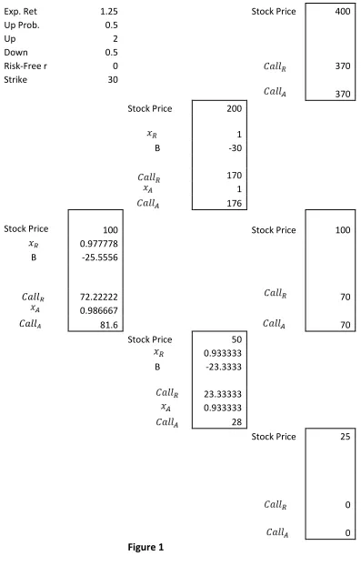
2.1 Analogy Making: A Two Period Binomial Example with Delta Hedging
Consider a two period binomial model. The parameters are: Up factor=2, Down factor=0.5, Current
stock price=$100, Risk free interest rate per binomial period=0, Strike price=$30, and the
probability of up movement=0.5. It follows that the expected gross return from the stock per
binomial period is 1.25 ( .
The call option can be priced both via analogy as well as via arbitrage argument. The
no-arbitrage price is denoted by whereas the analogy price is denoted by . Define and
where the differences are taken between the possible next period values that can be reached from a given node.
Figure 1 shows the binomial tree and the corresponding no-arbitrage and analogy prices.
Two things should be noted. Firstly, in the binomial case considered, before expiry, the analogy
price is always larger than the no-arbitrage price. Secondly, the delta hedging portfolios in the two
cases and grow at different rates. The portfolio grows at the rate
equal to the expected return on stock per binomial period (which is 1.25 in this case). In the analogy
case, the value of delta-hedging portfolio when the stock price is 100 is 17.06667
. In the next period, if the stock price goes up to 200, the value becomes 21.33333
. If the stock price goes down to 50, the value also ends up being equal to
21.33333 . That is, either way, the rate of growth is the same and is equal to
1.25 as . Similarly, if the delta hedging portfolio is constructed at any
other node, the next period return remains equal to the expected return from stock. It is easy to
verify that the portfolio grows at a different rate which is equal to the risk free rate per
11 The fact that the delta hedging portfolio under analogy making grows at a rate which is equal to the
perceived expected return on the underlying stock is used to derive the analogy based option pricing formulas
in continuous time in section 4. In the next section, the corresponding discrete time results are
presented. Note, as discussed earlier, the marginal investor in a call option is likely to be more
optimistic than the marginal investor in the underlying stock. In the context of the example
presented, this would mean that they perceive different binomial trees. Specifically, they would
perceive different up and down factors as up and down factors are a function of distribution of
12
Exp. Ret 1.25 Stock Price 400
Up Prob. 0.5
Up 2
Down 0.5
Risk-Free r 0 370
Strike 30
370
Stock Price 200
1
B -30
170 1 176
Stock Price 100 Stock Price 100
0.977778
B -25.5556
72.22222 70 0.986667
81.6 70
Stock Price 50
0.933333
B -23.3333
23.33333 0.933333 28
Stock Price 25
[image:13.612.73.470.69.702.2]13
3. Analogy Making: The Binomial Case
Consider a two state world. The equally likely states are Red, and Blue. There is a stock with prices corresponding to states Red, and Blue respectively, where . The state realization takes place at time . The current time is time . We denote the risk free discount rate by . That is,
there is a riskless zero coupon bond that has a price of B in both states with a price of
today. For simplicity and without loss of generality, we assume that and . The current
price of the stock is such that . We further assume that That is, the stock
price reflects a positive risk premium. In other words, where .
4 is the risk
premium reflected in the price of the stock.5 As we have assumed , it follows that
.
Suppose a new asset which is a European call option on the stock is introduced. By
definition, the payoffs from the call option in the two states are:
Where is the striking price, and are the payoffs from the call option corresponding to
Red, and Blue states respectively.
How much is an analogy maker willing to pay for this call option?
There are two cases in which the call option has a non-trivial price: 1) and 2)
The analogy maker infers the price of the call option, , by equating the expected return from the
call to the return he expects from holding the underlying stock:
4
In general, a stock price can be expressed as a product of a discount factor and the expected payoff if it follows a binomial process in discrete time (as assumed here), or if it follows a geometric Brownian motion in continuous time.
5
14 For case 1 ( ), one can write:
Substituting in (3.3):
The above equation is the one period analogy option pricing formula for the binomial case when call
remains in-the-money in both states.
The corresponding no-arbitrage price is (from the principle of no-arbitrage):
For case 2 ( , the analogy price is:
And, the corresponding no-arbitrage price is:
Proposition 1 The analogy price is larger than the corresponding no-arbitrage price if a
positive risk premium is reflected in the price of the underlying stock and there are no
transaction costs.
Proof.
15 Suppose there are transaction costs, denoted by “c”, which are assumed to be symmetric and
proportional. That is, if the stock price is S, a buyer pays and a seller receives .
Similar rule applies when the bond or the option is traded. That is, if the bond price is B, a buyer
pays and a seller receives . We further assume that the call option is cash settled.
That is, there is no physical delivery.
Introduction of the transaction cost does not change the analogy price as the expected
returns on call and on the underlying stock are proportionally reduced. However, the cost of
replicating a call option changes. The total cost of successfully replicating a long position in the call
option by buying the appropriate replicating portfolio and then liquidating it in the next period to
get cash (as call is cash settled) is:
The corresponding inflow from shorting the appropriate replicating portfolio to fund the
purchase of a call option is:
Proposition 2 shows that if transaction costs exist and the risk premium on the underlying stock is
within a certain range, the analogy price lies within the no-arbitrage interval. Hence, riskless profit
16
Proposition 2 In the presence of symmetric and proportional transaction costs, analogy
makers cannot be arbitraged out of the market if the risk premium on the underlying stock
satisfies:
Proof.
See Appendix B
▄
Intuitively, when transaction costs are introduced, there is no unique no-arbitrage price. Instead, a
whole interval of no-arbitrage prices comes into existence. Proposition 2 shows that for reasonable
parameter values, the analogy price lies within this no-arbitrage interval in a one period binomial
model. As more binomial periods are added, the transaction costs increase further due to the need
for additional re-balancing of the replicating portfolio. In the continuous limit, the total transaction
cost is unbounded. Reasonably, arbitrageurs cannot make money at the expense of analogy makers
in the presence of transaction costs ensuring that the analogy makers survive in the market.
It is interesting to consider the rate at which the delta-hedged portfolio grows under analogy
making. Proposition 3 shows that under analogy making, the delta-hedged portfolio grows at a rate
. This is in contrast with the Black Scholes Merton/Binomial Model in which the
17
Proposition 3 If analogy making determines the price of the call option, then the
corresponding delta-hedged portfolio grows with time at the rate of .
Proof.
See Appendix C ▄
Corollary 3.1 If there are multiple binomial periods then the growth rate of the delta-hedged
portfolio per binomial period is .
In continuous time, the difference in the growth rates of the delta-hedged portfolio under analogy
making and under the Black Scholes/Binomial model leads to an option pricing formula under
analogy making which is different from the Black Scholes formula. The continuous time formula is
presented in the next section.
4. Analogy Making: The Continuous Case
We maintain all the assumptions of the Black-Scholes model except one. We allow for transaction
costs whereas the transaction costs are ignored in the Black-Scholes model. As is well known,
introduction of the transaction costs invalidates the replication argument underlying the Black
Scholes formula. See Soner, Shreve, and Cvitanic (1995). As seen in the last section, transaction
costs have no bearing on the analogy argument as they simply reduce the expected return on the call
and on the underlying stock proportionally.
Proposition 4 shows the analogy based partial differential equation under the assumption
that the underlying follows geometric Brownian motion, which is the limiting case of the discrete
binomial model.We also explicitly allow for the possibility that different marginal investors
determine prices of calls with different strikes. This is reasonable as call buying is a bullish strategy
18
Proposition 4 If analogy makers set the price of a European call option, the analogy option
pricing partial differential Equation (PDE) is
Where is the risk premium that a marginal investor in the call option with strike ‘K’
expects from the underlying stock.
Proof.
See Appendix D
▄
Just like the Black Scholes PDE, the analogy option pricing PDE can be solved by transforming it
into the heat equation. Proposition 5 shows the resulting call option pricing formula for European
options without dividends under analogy making.
Proposition 5 The formula for the price of a European call is obtained by solving the
analogy based PDE. The formula is where
and
Proof.
See Appendix E.
▄
Corollary 5.1 The formula for the analogy based price of a European put option is
19 As proposition 5 shows, the analogy formula is exactly identical to the Black Scholes formula except
for the appearance of , which is the risk premium that a marginal investor in the call option with
strike K expects from the underlying stock. Note, that full allowance is made for the possibility that
such expectations vary with strike price as more optimistic investors are likely to self-select into
higher strike calls.
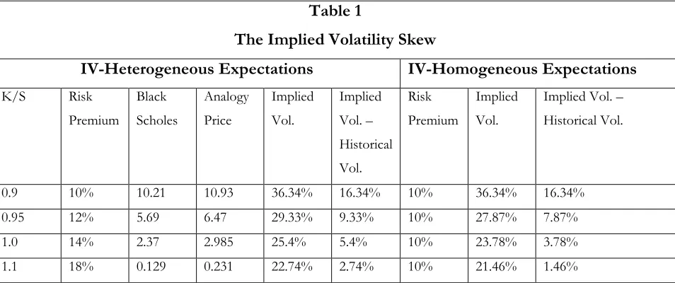
5. The Implied Volatility Skew
If analogy making determines option prices (formulas in proposition 5), and the Black Scholes
model is used to infer implied volatility, the skew is observed. Table 1 shows two examples of this. In the illustration titled “IV-Homogeneous Expectation”, the perceived risk premium on the underlying stock does not vary with the striking price. The other parameters are:
. In the illustration titled “IV-Heterogeneous Expectations”,
the risk premium on the underlying stock is varied by 40 basis points for every 0.01 change in
moneyness. That is, for a change of $5 in strike, the risk premium increases by 200 basis points. This
captures the possibility that more optimistic investors self-select into higher strike calls. Other
parameters are kept the same.
[image:20.612.71.548.460.660.2]Table 1
The Implied Volatility Skew
IV-Heterogeneous Expectations IV-Homogeneous Expectations
K/S Risk
Premium
Black
Scholes
Analogy
Price
Implied
Vol.
Implied
Vol. –
Historical
Vol.
Risk
Premium
Implied
Vol.
Implied Vol. –
Historical Vol.
0.9 10% 10.21 10.93 36.34% 16.34% 10% 36.34% 16.34%
0.95 12% 5.69 6.47 29.33% 9.33% 10% 27.87% 7.87%
1.0 14% 2.37 2.985 25.4% 5.4% 10% 23.78% 3.78%
20 As Table 1 shows, the implied volatility skew can be observed with both homogeneous and
heterogeneous expectations. It also shows that the difference between implied volatility and realized
volatility is higher with heterogeneous expectations. It is easy to see that higher the dispersion in
beliefs, greater is the difference between implied and realized volatilities (as long as more optimistic
investors self-select into higher strike calls). This is consistent with empirical evidence that shows
that higher the dispersion in beliefs, greater is the difference between implied and realized volatilities
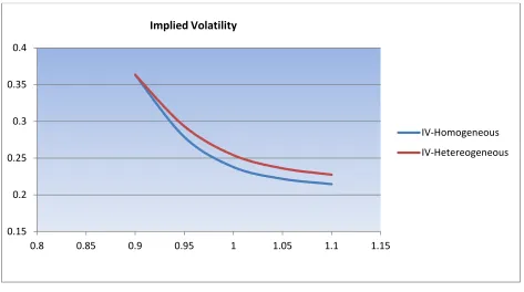
[image:21.612.72.545.221.485.2](see Beber A., Breedan F., and Buraschi A. (2010)). Figure 2 is a graphical illustration of Table 1.
Figure 2
It is easy to illustrate that, with analogy making, the implied volatility skew gets flatter as time to
expiry increases. As an example, with underlying stock price=$100, volatility=20%, risk premium on
the underlying stock=5%, and the risk free rate of 0, the flattening with expiry can be seen in Figure
3. Hence, the implications of analogy making are consistent with key observed features of the
structure of implied volatility skew. 0.15
0.2 0.25 0.3 0.35 0.4
0.8 0.85 0.9 0.95 1 1.05 1.1 1.15
IV-Homogeneous
IV-Hetereogeneous
21
Figure 3
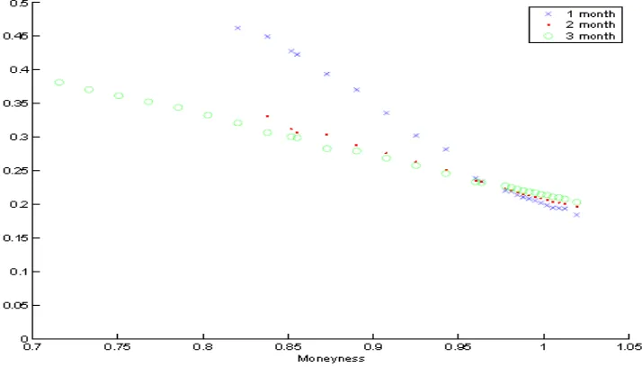
As an illustration of the fact that implied volatility curve flattens with expiry, Figure 4 is a
reproduction of a chart from Fouque, Papanicolaou, Sircar, and Solna (2004) (Figure 2 from their
paper). It plots implied volatilities from options with at least two days and at most three months to
expiry. The flattening is clearly seen.
Figure 4 Implied volatility as a function of moneyness on January 12, 2000, for options with at least two days and
at most three months to expiry.
10 15 20 25 30 35 40 45 50 55 60
0.7 0.8 0.9 1 1.1
Expiry=0.06 Year
Expiry=1 Year Implied Volatility
[image:22.612.97.454.458.667.2]22 So far, we have only considered analogy making as the sole mechanism generating the skew.
Stochastic volatility and jump diffusion are other popular methods that give rise to the skew. In
sections 8 and 9, we show that analogy making is complementary to stochastic volatility and jump
diffusion models by integrating analogy making with the models of Hull and White (1987) and
Merton (1976) respectively. In the next section, the profitability of covered call writing and zero-beta
straddles is examined in the analogy model.
6. The Profitability of Covered Call Writing with Analogy Making
The profitability of covered call writing is quite puzzling in the Black Scholes framework. Whaley
(2002) shows that BXM (a Buy Write Monthly Index tracking a Covered Call on S&P 500) has
significantly lower risk when compared with the index, however, it offers nearly the same return as
the index. Similar conclusions are reached in studies by Feldman and Roy (2004) and Callan
Associates (2006). In the Black Scholes framework, the covered call strategy is expected to have
lower risk as well as lower return when compared with buying the index only. See Black (1975). In
fact, in an efficient market, the risk adjusted return from covered call writing should be no different
than the risk adjusted return from just holding the index.
The covered call strategy (S denotes stock, C denotes call) is given by:
With analogy making, this is equal to:
(6.1)
The corresponding value under the Black Scholes assumptions is:
(6.2)
A comparison of 6.1 and 6.2 shows that covered call strategy is expected to perform much
better with analogy making when compared with its expected performance in the Black Scholes
23 the stock and a weight of on a hypothetical risk free asset with a return of . The stock
has a return of plus dividend yield. This implies that, with analogy making, the return from
covered call strategy is expected to be comparable to the return from holding the underlying stock
only. The presence of a hypothetical risk free asset in 6.1 implies that the standard deviation of
covered call returns is lower than the standard deviation from just holding the underlying stock.
Hence, the superior historical performance of covered call strategy is no mystery if call prices are
determined via analogy making.
6.1 The Zero-Beta Straddle Performance with Analogy Making
Another empirical puzzle in the Black-Scholes/CAPM framework is that zero beta straddles lose
money. Goltz and Lai (2009), Coval and Shumway (2001) and others find that zero beta straddles
earn negative returns on average. This is in sharp contrast with the Black-Scholes/CAPM prediction
which says that the zero-beta straddles should earn the risk free rate. A zero-beta straddle is
constructed by taking a long position in corresponding call and put options with weights chosen so
as to make the portfolio beta equal to zero:
Where and
It is straightforward to show that with analogy making, where call and put prices are
determined in accordance with proposition 5, the zero-beta straddle earns a significantly smaller
return than the risk free rate with returns being negative for a wide range of realistic parameter
values. Hence, the observed empirical performance of zero-beta straddle is no puzzle with analogy
based option pricing. Intuitively, with analogy making, both call and put options are more expensive
when compared with Black-Scholes prices. Hence, the returns are smaller.
Analogy based option pricing not only generates the implied volatility skew, it is also
consistent with key empirical findings regarding option portfolio returns such as covered call writing
24
7. Leverage Adjusted Option Returns with Analogy Making
Leverage adjustment dilutes beta risk of an option by combining it with a risk free asset. Leverage
adjustment combines each option with a risk-free asset in such a manner that the overall beta risk
becomes equal to the beta risk of the underlying stock. The weight of the option in the portfolio is equal to its inverse price elasticity w.r.t the underlying stock’s price:
where (i.e price elasticity of call w.r.t the underlying stock)
Constantinides, Jackwerth and Savov (2013) uncover a number of puzzling empirical facts
regarding leverage adjusted index option returns. They find that over a period ranging from April
1986 to January 2012, the average percentage monthly returns of leverage-adjusted index call and put
options are decreasing in the ratio of strike to spot. They also find that leverage adjusted put returns are larger than
the corresponding leverage adjusted call returns. The empirical findings in Contantinides et al (2012) are
inconsistent with the Black-Scholes/CAPM framework, which predicts that the leverage adjusted
returns should be equal to the return from the underlying index. That is, they should not fall with
strike, and the leverage adjusted put option returns should not be any different than the leverage
adjusted call returns.
If analogy making determines call prices, then the behavior of leverage adjusted call and put
returns should be a lot different than their predicted behavior under the Black-Scholes assumptions.
For call options:
(7.1)
where
25 According to the analogy based PDE:
(7.3)
Substituting (7.3) and (7.2) in (7.1) and simplifying leads to:
(7.4)
rises as the ratio of strike to spot increases. So, the leverage adjusted call option return must fall as
the ratio of strike to spot increases. Hence, analogy based option pricing is consistent with empirical
evidence. The corresponding leverage adjusted put option return with analogy based option pricing
is:
(7.5)
The term in brackets,
, falls as the ratio of strike to spot increases. Furthermore, (7.5) is
larger than (7.4). That is, the leverage adjusted put returns must fall as the ratio of strike to spot
increases and are also larger than the corresponding leverage adjusted call returns. Hence, empirical
findings in Constantinides et al (2012) regarding leverage adjusted option returns are consistent with
analogy based option pricing.
8. Analogy based Option Pricing with Stochastic Volatility
In this section, we put forward an analogy based option pricing model for the case when the
underlying stock price and its instantaneous variance are assumed to obey the uncorrelated
stochastic processes described in Hull and White (1987):
26 Where (Instantaneous variance of stock’s returns), and and are non-negative constants. and are standard Guass-Weiner processes that are uncorrelated. Time subscripts in and are suppressed for notational simplicity. If , then the instantaneous variance is a constant, and
we are back in the Black-Scholes world. Bigger the value of , which can be interpreted as the
volatility of volatility parameter, larger is the departure from the constant volatility assumption of the
Black-Scholes model.
Hull and White (1987) is among the first option pricing models that allowed for stochastic
volatility. A variety of stochastic volatility models have been proposed including Stein and Stein
(1991), and Heston (1993) among others. Here, we use Hull and White (1987) assumptions to show
that the idea of analogy making is easily combined with stochastic volatility. Clearly, with stochastic
volatility it does not seem possible to form a hedge portfolio that eliminates risk completely. This is
because there is no asset which is perfectly correlated with .
If analogy making determines call prices and the underlying stock and its instantaneous
volatility follow the stochastic processes described above, then the European call option price (no
dividends on the underlying stock for simplicity) must satisfy the partial differentiation equation
given below (see Appendix F for the derivation):
Where is the risk premium that a marginal investor in the call option expects to get from the
underlying stock.
By definition, under analogy making, the price of the call option is the expected terminal
value of the option discounted at the rate which the marginal investor in the option expects to get
from investing in the underlying stock. The price of the option is then:
Where the conditional distribution of as perceived by the marginal investor is such that
27 By defining as the means variance over the life of the option, the
distribution of can be expressed as:
Substituting (8.3) in (8.2) and re-arranging leads to:
By using an argument that runs in parallel with the corresponding argument in Hull and White
(1987), it is straightforward to show that the term inside the square brackets is the analogy making
price of the call option with a constant variance . Denoting this price by , the price of
the call option under analogy making when volatility is stochastic (as in Hull and White (1987)) is
given by (proof available from author):
Where
;
Equation (8.5) shows that the analogy based call option price with stochastic volatility is the analogy
based price with constant variance integrated with respect to the distribution of mean volatility.
8.1 Option Pricing Implications
Stochastic volatility models require a strong correlation between the volatility process and the stock
price process in order to generate the implied volatility skew. They can only generate a more
symmetric U-shaped smile with zero correlation as assumed here. In contrast, the analogy making
stochastic volatility model (equation 8.5) can generate a variety of skews and smiles even with zero
correlation. What type of implied volatility structure is ultimately seen depends on the parameters
28 and , only a more symmetric smile arises. For positive , there is a threshold value of below which skew arises and above which smile takes shape. Typically, for options on individual
stocks, the smile is seen, and for index options, the skew arises. The approach developed here
provides a potential explanation for this as is likely to be lower for indices due to inbuilt
diversification (giving rise to skew) when compared with individual stocks.
9. Analogy based Option Pricing with Jump Diffusion
In this section, we integrate the idea of analogy making with the jump diffusion model of Merton
(1976). As before, the point is that the idea of analogy making is independent of the distributional
assumptions that are made regarding the behavior of the underlying stock. In the previous section,
analogy making is combined with the Hull and White stochastic volatility model to illustrate the
same point.
Merton (1976) assumes that the stock returns are a mixture of geometric Brownian motion and
Poisson-driven jumps:
Where is a standard Guass-Weiner process, and is a Poisson process. and are
assumed to be independent. is the mean number of jump arrivals per unit time,
where is the random percentage change in the stock price if the Poisson event occurs, and
is the expectations operator over the random variable . If (hence, ) then the stock
price dynamics are identical to those assumed in the Black Scholes model. For simplicity, assume
that .
The stock price dynamics then become:
Clearly, with jump diffusion, the Black-Scholes no-arbitrage technique cannot be employed
as there is no portfolio of stock and options which is risk-free. However, with analogy making, the
price of the option can be determined as the return on the call option demanded by the marginal
29 If analogy making determines the price of the call option when the underlying stock price
dynamics are a mixture of a geometric Brownian motion and a Poisson process as described earlier,
then the following partial differential equation must be satisfied (see Appendix G for the derivation):
If the distribution of is assumed to log-normal with a mean of 1 (assumed for simplicity)
and a variance of then by using an argument analogous to Merton (1976), the following analogy
based option pricing formula for the case of jump diffusion is easily derived (proof available from
author):
and
Where is the fraction of volatility explained by jumps.
The formula in (9.2) is identical to the Merton jump diffusion formula except for one parameter, ,
which is the risk premium that a marginal investor in the call option expects from the underlying
stock.
9.1 Option Pricing Implications
Merton’s jump diffusion model with symmetric jumps (jump mean equal to zero) can only produce a symmetric smile. Generating the implied volatility skew requires asymmetric jumps (jump mean
30 generated even when jumps are symmetric. In particular, for low values of , a more symmetric
smile is generated, and for larger values of skew arises.
Even if we one assumes an asymmetric jump distribution around the current stock price,
Merton formula, when calibrated with historical data, generates a skew which is a lot less
pronounced (steep) than what is empirically observed. See Andersen and Andreasen (2002). The
skew generated by the analogy formula (with asymmetric jumps) is typically more pronounced
(steep) when compared with the skew without analogy making. Hence, analogy making potentially
adds value to a jump diffusion model.
If prices are determined in accordance with the formula given in (9.2) and the Black Scholes
formula is used to back-out implied volatility, the skew is observed. As an example, Figure 5 shows
the skew generated by assuming the following parameter values:
.
In Figure 5, the x-axis values are various values of strike/spot, where spot is fixed at 100. Note, that
the implied volatility is always higher than the actual volatility of 25%. Empirically, implied volatility
is typically higher than the realized or historical volatility. As one example, Rennison and Pederson
(2012) use data ranging from 1994 to 2012 from eight different option markets to calculated implied
volatility from at-the-money options. They report that implied volatilities are typically higher than
realized volatilities.
Figure 5
0 10 20 30 40 50 60 70
0.6 0.7 0.8 0.9 1 1.1 1.2 1.3 1.4
Implied Volatility Skew with Risk Premium=5%
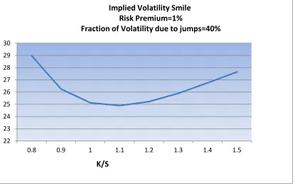
31 In general, in the jump diffusion analogy model, the skew generated turns into a smile as the risk
premium on the underlying falls (approaches the risk-free rate). Figure 6 shows one instance when
the risk premium is 1% and fraction of volatility due to jumps is 40% (all other parameters are kept
[image:32.612.74.489.169.431.2]the same).
Figure 6
10. Conclusions
The observation that people tend to think by analogies and comparisons has important implications
for option pricing that are thus far ignored in the literature. Prominent cognitive scientists argue that
analogy making is the way human brain works (Hofstadter and Sander (2013)). There is strong
experimental evidence that a call option is valued in analogy with the underlying stock (see
Rockenbach (2004), Siddiqi (2012), and Siddiqi (2011)). A call option is commonly considered to be
a surrogate for the underlying stock by experienced market professionals, which lends further
support to the idea of analogy based option valuation. In this article, the notion that a call option is
valued in analogy with the underlying stock is explored and the resulting option pricing model is put
forward. The analogy option pricing model provides a new explanation for the implied volatility
skew puzzle. The analogy based explanation complements the existing explanation as it is possible to 22
23 24 25 26 27 28 29 30
0.8 0.9 1 1.1 1.2 1.3 1.4 1.5
Implied Volatility Smile Risk Premium=1%
Fraction of Volatility due to jumps=40%
32 integrate analogy making with stochastic volatility and jump diffusion approaches. The paper does
that and puts forward analogy based option valuation models with stochastic volatility and jumps
respectively. In contrast with other stochastic volatility and jump diffusion models in the literature,
analogy making stochastic volatility model generates the skew even when there is zero correlation
between the stock price and volatility processes, and analogy based jump diffusion can produce the
skew even with symmetric jumps.
The analogy model differs minimally from the Black Scholes model due to the introduction
of one additional variable. The additional variable captures the risk premium (subjective) that the
marginal call option investor expects to get from the underlying stock. It is surprising that such a
minimally different model can explain a wide variety of phenomena such as implied volatility skew,
leverage adjusted option returns, superior performance of covered call writing, and
33
References
Amin, K. (1993). “Jump diffusion option valuation in discrete time”,Journal of Finance 48, 1833-1863.
Anderson, Torben, Luca Benzoni, and Jesper Lund (2002). “An empirical investigation of continuous time equity return models”, Journal of Finance 57, 1239–1284.
Bakshi G., Cao, C., Chen, Z. (1997). “Empirical performance of alternative option pricing models”,Journal of
Finance 52, 2003-2049.
Ball, C., Torous, W. (1985). “On jumps in common stock prices and their impact on call option pricing”,
Journal of Finance 40, 155-173.
Bates, D. (2000), “Post-‘87 Crash fears in S&P 500 futures options”, Journal of Econometrics, 94, pp. 181-238.
Beber A., Breedan F., and Buraschi A. (2010), “Differences in beliefs and currency risk premiums”, Journal of
Financial Economics, Vol. 98, Issue 3, pp. 415-438.
Black, F., Scholes, M. (1973). “The pricing of options and corporate liabilities”. Journal of Political Economy 81(3): pp. 637-65
Bollen, N., and Whaley, R. (2004). “Does Net Buying Pressure Affect the Shape of Implied Volatility Functions?” Journal of Finance 59(2): 711–53
Chernov, Mikhail, Ron Gallant, Eric Ghysels, and George Tauchen, 2003, Alternative models of stock price dynamics, Journal of Econometrics 116, 225–257.
Christensen B. J., and Prabhala, N. R. (1998), “The Relation between Realized and Implied Volatility”, Journal
of Financial Economics Vol.50, pp. 125-150.
Constantinides, G. M., Jackwerth, J. C., and Savov, A. (2013), “The Puzzle of Index Option Returns”,Review of Asset Pricing Studies.
Coval, J. D., and Shumway, T. (2001), “Expected Option Returns”, Journal of Finance, Vol. 56, No.3, pp. 983-1009.
Derman, E. (2003), “The Problem of the Volatility Smile”, talk at the Euronext Options Conference available
at http://www.ederman.com/new/docs/euronext-volatility_smile.pdf
Derman, E, (2002), “The perception of time, risk and return during periods of speculation”.
Quantitative Finance Vol. 2, pp. 282-296.
Derman, E., Kani, I., & Zou, J. (1996), “The local volatility surface: unlocking the information in index option prices”, Financial Analysts Journal, 52, 4, 25-36
Derman, E., Kani, I. (1994), “Riding on the Smile.” Risk, Vol. 7, pp. 32-39
Duan, Jin-Chuan, and Wei Jason (2009), “Systematic Risk and the Price Structure of Individual Equity Options”, The Review of Financial studies, Vol. 22, No.5, pp. 1981-2006.
34 Dumas, B., Fleming, J., Whaley, R., 1998. Implied volatility functions: empirical tests. Journal of Finance 53, 2059-2106.
Dupire, B. (1994), “Pricing with a Smile”, Risk, Vol.7, pp. 18-20
Emanuel, D. C., and MacBeth, J. D. (1982), “Further Results on the Constant Elasticity of Variance Option Pricing Model”, Journal of Financial and Quantitative Analysis, Vol. 17, Issue 4, pp. 533-554.
Fouque, Papanicolaou, Sircar, and Solna (2004), “Maturity Cycles in Implied Volatility” Finance and Stochastics, Vol. 8, Issue 4, pp 451-477
Gilboa, I., Schmeidler, D. (2001), “A Theory of Case Based Decisions”. Publisher: Cambridge University Press.
Goltz, F., and Lai, W. N. (2009), “Empirical properties of straddle returns”, The Journal of Derivatives, Vol. 17, No. 1, pp. 38-48.
Han, B. (2008), “Investor Sentiment and Option Prices”, The Review of Financial Studies, 21(1), pp. 387-414.
Heston S., Nandi, S., 2000. A closed-form GARCH option valuation model. Review of Financial Studies 13, 585-625.
Heston S., 1993. “A closed form solution for options with stochastic volatility with application to bond and currency options. Review of Financial Studies 6, 327-343.
Hodges, S. D., Neuberger, A. (1989), “Optimal replication of contingent claims under transaction costs”, The
Review of Futures Markets 8, 222–239
Hofstadter, D., and Sander, E. (2013), “Surfaces and Essences: Analogy as the fuel and fire of thinking”, Published by Basic Books, April.
Hull, J., White, A., 1987. The pricing of options on assets with stochastic volatilities. Journal of Finance 42, 281-300.
Jackwerth, J. C., (2000), “Recovering Risk Aversion from Option Prices and Realized Returns”, The Review of
Financial Studies, Vol. 13, No, 2, pp. 433-451.
Jehiel, P. (2005), “Analogy based Expectations Equilibrium”,Journal of Economic Theory, Vol. 123, Issue 2, pp. 81-104.
Lakonishok, J., I. Lee, N. D. Pearson, and A. M. Poteshman, 2007, “Option Market Activity,”
Review of Financial Studies, 20, 813-857.
Melino A., Turnbull, S., 1990. “Pricing foreign currency options with stochastic volatility”. Journal of Econometrics 45, 239-265
Miyahara, Y. (2001), “Geometric Levy Process & MEMM Pricing Model and Related Estimation Problems”, Asia-Pacific Financial Markets 8, 45–60 (2001)
Mullainathan, S., Schwartzstein, J., & Shleifer, A. (2008) “Coarse Thinking and Persuasion”. The Quarterly
Journal of Economics, Vol. 123, Issue 2 (05), pp. 577-619.
35 Rennison, G., and Pedersen, N. (2012)“The Volatility Risk Premium”, PIMCO, September.
Rockenbach, B. (2004), “The Behavioral Relevance of Mental Accounting for the Pricing of Financial Options”. Journal of Economic Behavior and Organization, Vol. 53, pp. 513-527.
Rubinstein, M., 1994. Implied binomial trees. Journal of Finance 49, 771-818.
Schwert W. G. (1990), “Stock volatility and the crash of 87”. Review of Financial Studies 3, 1 (1990), pp. 77–102 Siddiqi, H. (2009), “Is the Lure of Choice Reflected in Market Prices? Experimental Evidence based on the 4-Door Monty Hall Problem”. Journal of Economic Psychology, April.
Siddiqi, H. (2011), “Does Coarse Thinking Matter for Option Pricing? Evidence from an Experiment” IUP
Journal of Behavioral Finance, Vol. VIII, No.2. pp. 58-69
Siddiqi, H. (2012), “The Relevance of Thinking by Analogy for Investors’ Willingness to Pay: An Experimental Study”, Journal of Economic Psychology, Vol. 33, Issue 1, pp. 19-29.
Soner, H.M., S. Shreve, and J. Cvitanic, (1995), “There is no nontrivial hedging portfolio for option pricing with transaction costs”, Annals of Applied Probability 5, 327–355.
Stein, E. M., and Stein, J. C (1991) “Stock price distributions with stochastic volatility: An analytic approach”
Review of Financial Studies, 4(4):727–752.
Wiggins, J., 1987. Option values under stochastic volatility: theory and empirical estimates. Journal of Financial Economics 19, 351-372.
Appendix A
Proof of Proposition 1
For case 1, when , the results follow from a direct comparison of (3.4) and (3.5).
For case 2, when , the spectrum of possibilities is further divided into three sub-classes
and the results are proved for each sub-class one by one. The three sub-classes are: (i) ,
(ii) , and (iii) .
Case 2 sub-class (i):
If we assume that , we arrive at a contradiction as follows:
Substitute and above and simplify, it follows that , which is a
36
Case 2 sub-class (ii): or equivalently where
If we assume that , we arrive at a contradiction as follows:
Substitute and above and simplify, it follows that , which is a
contradiction.
Case 2 sub-class (iii): or equivalently where
Similar logic as used in the case above leads to a contradiction: .
Hence, the analogy price must be larger than the no-arbitrage price if the risk premium is positive
and there are no transaction costs.
Appendix B
Proof of Proposition 2
If then there is no-arbitrage if the following holds:
Realizing that and simplifying
leads to inequality (3.12).
If then there is no-arbitrage if the following holds:
Realizing that
37
And simplifying
leads to (3.1).
Appendix C
Proof of Proposition 3
Case 1:
Delta-hedged portfolio is . In this case, , , and
If the red state is realized, changes from to . If the blue state is realized also
changes from to . Hence, the growth rate is equal to in either state.
Case 2:
Delta-hedged portfolio is In this case,
,
, and
Consider three sub-classes and prove the result for each: (i) , (ii) , and
(iii) For the first sub-class the delta-hedged portfolio changes from the initial value
of to in both the red and the blue states. Hence, the growth rate is equal to in either
state. For the second and third sub-classes, the delta-hedged portfolio changes from
to
in both red and blue states. Hence, the growth rate is equal to
.
Appendix D
In the binomial analogy case, the delta-hedged portfolio grows at the rate . Divide
38
Where and by Ito’s Lemma
The above is the analogy based PDE.
Appendix E
The analogy based PDE derived in Appendix D can be solved by converting to heat equation and
exploiting its solution. The steps are identical to the derivation of the Black Scholes model with the
risk free rate , replaced with .
Appendix F
Start by considering the value of a delta hedged portfolio: .
Over a small time interval, :
(F1)
39
(F2)
Substituting (F2) in (F1) and re-arranging:
(F3)
Choosing , and realizing that, with analogy making, , (F3) becomes:
(F4)
(F4) simplifies to:
(F5)
Appendix G
By following a very similar argument as in appendix F, and using Ito’s lemma for the continuous part and an analogous Lemma for the discontinuous part, the following is obtained: