1
2
Detection of selective sweeps in structured populations: a comparison of
3recent methods
45
Alexandra I. Vatsiou
1,2, Eric Bazin
1, Oscar E. Gaggiotti
1,26
7
1Laboratoire d'Ecologie Alpine, UMR CNRS 5553, Université Joseph Fourier, Grenoble, France 8
2Scottish Oceans Institute, East Sands, University of St Andrews, St Andrews, 9
KY16 8LB, UK
10
*Corresponding author: E-mail: [email protected] 11
keywords: positive selection, haplotype structure, genome scan methods, accuracy
12
13
14
16
Abstract
17
Identifying genomic regions targeted by positive selection has been a longstanding
18
interest of evolutionary biologists. This objective was difficult to achieve until the recent
19
emergence of Next Generation Sequencing, which is fostering the development of large-scale
20
catalogs of genetic variation for increasing number of species. Several statistical methods have
21
been recently developed to analyze these rich datasets but there is still a poor understanding of
22
the conditions under which these methods produce reliable results. This study aims at filling this
23
gap by assessing the performance of genome-scan methods that consider explicitly the physical
24
linkage among SNPs surrounding a selected variant. Our study compares the performance of
25
seven recent methods for the detection of selective sweeps (iHS, nSL, EHHST, xp-EHH,
XP-26
EHHST, XPCLR and hapFLK). We use an individual-based simulation approach to investigate
27
the power and accuracy of these methods under a wide range of population models under both
28
hard and soft sweeps. Our results indicate that XPCLR and hapFLK perform best and can detect
29
soft sweeps under simple population structure scenarios if migration rate is low. All methods
30
perform poorly with moderate to high migration rates, or with weak selection and very poorly
31
under a hierarchical population structure. Finally, no single method is able to detect both starting
32
and nearly completed selective sweeps. However, combining several methods (XPCLR or
33
hapFLK with iHS or nSL) can greatly increase the power to pinpoint the selected region.
34
35
Introduction
37
Population geneticists and evolutionary biologists have a longstanding interest in understanding
38
the ecological and genetic mechanisms that allow species to adapt to local environmental
39
conditions. The recent advent of Next Generation Sequencing (NGS) (Shendure & Ji 2008) and
40
the high density SNP arrays it generates has allowed rapid advances in this field and has fostered
41
the emergence of the population genomics approach (Luikart et al. 2003). This new paradigm is
42
focused on the use of genome-wide data to distinguish between locus-specific effects (mainly
43
selection but also mutation, and recombination) and genome-wide effects such as genetic drift. It
44
has proven particularly useful to detect signatures of selection, and has been used to uncover
45
genes involved in local adaptation, disease susceptibility, resistance to pathogens, and other
46
phenotypic traits of interest to plant and animal breeders.
47
At the genetic level, local adaptation involves a process whereby directional selection
48
induced by local environmental conditions will favor the spread of genetic variants associated
49
with beneficial phenotypic traits. If selection is strong at the level of an individual locus the
50
selected variant will increase in frequency. Additionally, selection will modify the pattern of
51
diversity around the selected locus through genetic hitchhiking (Barton 2000; Smith & Haigh
52
1974). This process, known as a selective sweep, has been extensively studied using models of
53
isolated populations (Hermisson & Pennings 2005; Pennings & Hermisson 2006a, b; Kim &
54
Nielsen 2004; Sabeti et al. 2002; Smith & Haigh 1974; Voight et al. 2006) but much less studied
55
under structured population scenarios. In this latter case, analyses focused on either, an
56
universally favoured mutation that spreads from its deme of origin to other demes (Barton 2000;
57
Bierne 2010; Slatkin & Wiehe 1998) or on a scenario where the new selected variant is favoured
in one part of the species range but counter selected in the other half (Bierne 2010). However,
59
there is a third scenario still poorly understood but frequently assumed by studies of local
60
adaptation, particularly in humans. Under this scenario, a selected variant is favoured in one part
61
of the species range and is neutral elsewhere (e.g. lactase persistence, skin pigmentation, high
62
altitude adaptation; Jeong & Di Rienzo 2014).
63
Several so-called “genome-scan methods’ have been proposed for the detection of
64
positive selection from dense SNP maps. The most widely used and thoroughly evaluated type of
65
methods is based on Lewontin and Krakauer (1973) approach and is focused on single-locus FST
66
(Beaumont & Balding 2004; Beaumont & Nichols 1996; Foll & Gaggiotti 2008). These methods
67
implicitly or explicitly assume that SNPs are physically unlinked and are most effective when
68
neutral genetic differentiation is low (Price et al. 2008) and/or when the selective sweep is close
69
to fixation (Pickrell et al. 2009). Other methods are specifically aimed at detecting selective
70
sweeps by focusing on the distribution of genetic variation along a chromosome within a
71
population when selection is acting, as predicted by the theory of genetic hitchhiking (Fay & Wu
72
2000; Kim & Stephan 2002; Nielsen et al. 2005). These methods are applicable to isolated
73
populations and their behavior has been extensively studied (Jensen et al. 2005, Zang et al. 2005,
74
Zeng et al. 2007).
75
A third type of genome scan methods considers explicitly the physical linkage among
76
SNPs surrounding a selected variant, either by focusing on patterns of long-range haplotype
77
homozygosity (Sabeti et al. 2002; Voight et al. 2006) or by modelling the effect of linkage on
78
multilocus genetic differentiation (Chen et al. 2010). These methods are more recent and their
79
properties have not been extensively investigated. Moreover, although they are focused on either
80
a single population (Ferrer-Admetlla et al. 2014; Sabeti et al. 2002; Voight et al. 2006) or on
pairs of populations (Chen et al. 2010; Fariello et al. 2013; Sabeti et al. 2007), they are being
82
used to study structured populations consisting of many subpopulations without a clear
83
understanding of how migration and complex population structure may affect their power and
84
error rates. Thus, the objective of the present study is to carry out a thorough evaluation of the
85
performance of these methods under various scenarios of population structure. We focus mainly
86
on the case where the selected variant is beneficial in part of the species range and neutral
87
elsewhere, as it is the underlying scenario envisaged by many recent studies of adaptation (Foll et
88
al. 2014; Hancock et al. 2008; Lao et al. 2007). Additionally we consider both hard and soft
89
selective sweeps. These two scenarios differ in the origin of the selected variant. In a hard
90
selective sweep the favoured allele appears through de novo mutation while in a soft sweep it is
91
already segregating at low frequency in the population (standing genetic variation) or it arises
92
from recurrent mutations (Hermisson & Pennings 2005; Pennings & Hermisson 2006a, b;
93
Pritchard et al. 2010).
94
In the present analysis we compare the performance of seven recent methods to detect
95
selective sweeps. We incorporate in the analysis, methods that were developed to study a single
96
population, a pair of populations or multiple populations. We explain in detail the ability of each
97
method to capture the signal of selection left by both hard and soft sweeps under different
98
scenarios of structured populations and a range of parameter values (migration and selection).
99
The principle is to examine these methods on the same simulated datasets and draw conclusions
100
about how the different model parameters affect their performance as described by power and
101
false discovery rate. The goal of this analysis is to guide scientists in the choice of the methods
102
that is better suited for their biological model.
103
Material and Methods
105
Genome Scan Methods
106We focus our study on seven methods for which software is readily available: Integrated
107
Haplotype Score (iHS) (Voight et al. 2006), Number of Segregating sites by Length (nSL)
108
(Ferrer-Admetlla et al. 2014), Extended Haplotype-based Homozygosity Score Test (EHHST)
109
(Zhong et al. 2010), Cross Population Extended Haplotype Homozygosity (xp-EHH) (Sabeti et
110
al. 2007), Cross-population extended haplotype-based homozygosity score test (xp-EHHST)
111
(Zhong et al. 2011), Cross population Composite Likelihood Ratio (XPCLR) (Chen et al. 2010)
112
and hapFLK (Fariello et al. 2013). They all use SNP data but propose different statistics to detect
113
selection. In what follows we will highlight their main differences but we also include more
114
technical details about all these methods in SI.
115
The methods we evaluate use different summary statistics that try to capture different
116
genetic patterns consistent with the action of positive selection. We can distinguish three groups
117
of methods:
118
(i) Methods based on the decay of haplotype homozygosity as a function of recombination
119
distance (iHS, nSL and xp-EHH): the underlying rationale of these methods is that selected
120
alleles will have unusually long range linkage disequilibrium given their frequency in the
121
population.
122
(ii) Methods based on the decay of genotype homozygosity around a target SNP (EHHST and
xp-123
EHHST): the underlying rationale is similar to that of the previous group but in this case
124
homozygosity is measured in terms of mean homozygosity across all individuals in the sample
instead of homozygosity of a region with respect to all chromosomes in the sample as in the
126
previous group.
127
(iii) Methods based on the extent of multilocus genetic differentiation among populations around
128
a target SNP (XPCLR and hapFLK): the underlying rationale is that genetic differentiation
129
around a selected variant will be much larger than expected under drift but instead of using
130
single-locus measures of differentiation it calculates differentiation for all SNPs within a
131
window centered around the target SNP.
132
Another important difference between methods lies in whether or not they require phased
133
data and information on the ancestral/derived status at each segregating site. XPCLR is the only
134
method that does not have these requirements. Finally, one last difference among methods that
135
needs to be highlighted refers to the number of populations they consider. iHS, nSL and EHHST
136
are focused on a single population, xp-EHH, xp-EHHST, XPCLR consider two populations,
137
while hapFLK considers an arbitrary number of populations.
138
139
Calculation of p values
140The first step in the comparison of several methods is to define a common framework for
141
assessing significance, which then allows us to calculate false positive and false negative rates as
142
well as power. We used two alternative approaches:
143
(a) From the empirical distribution of test scores: in this case, we calculate the test statistic for all
144
SNPs in the sample. Then using the empirical distribution of test scores, we consider as
145
potentially adaptive all the loci with scores falling in the outlying 5% of the distribution. In the
146
context of a simulation study, we know the truth and, therefore, we can readily identify true
and false positives across all synthetic samples so as to calculate error rates and power of each
148
method.
149
(b) From a distribution of tests scores generated by neutral simulations: in this case, we generate a
150
large number of synthetic datasets assuming a particular demographic history (deemed
151
appropriate for the species under study) and calculate the statistic scores for a target SNP. The
152
distribution of test scores is then used as the null distribution and any loci with a test score
153
falling in the outlying 5% of the distribution is considered potentially selected. In order to
154
compare he performance of the different methods, we also carried out simulations under
155
different selection scenarios and then pooled neutral and selected replicates to estimate power
156
at various false positive rates. These results are then presented as ROC curves obtained using
157
the R package “ROCR” (Sing et al. 2005).
158
The most widespread approach to assess significance when analysing real data is based on
159
the empirical distribution (approach a). The reason for this is that in most cases we do not know
160
with certainty the true demographic history of the species under study. Thus, we present the
161
results of this procedure in the main text and the results of the second procedure in the
162
supplementary information.
163
164
Simulations
165We generated synthetic data using SimuPOP (Peng & Amos 2008; Peng et al. 2011), a
general-166
purpose, individual-based simulation platform for forward-in-time population genetics modelling.
167
The Python scripts used to carry out the simulations are available at GitHub
168
(https://github.com/alexvat/simulations).
Initially, we simulated three different population structure scenarios, an island model
170
(Wright 1990), a stepping stone model (Kimura 1953) and a dichotomous population fission
171
model that leads to a hierarchical island structure (Figure S1). In these cases, we considered four
172
diploid demes, each of constant effective population size Ne = 2500. Thus, total population size
173
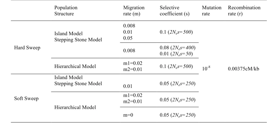
was 10,000. Table 1 presents a summary of the parameters that were used in the simulations. In
174
the case of the island and the stepping-stone models, every individual migrates to another deme
175
with probability m (0.05, 0.01 or 0.008). In the case of the hierarchical model, migration between
176
demes within the same group (continent) was higher than migration between demes in different
177
groups (see Figure S1c). In this latter scenario, we start at t = 0 with a single population (Z with
178
10,000 individuals). At t = 100 generations, it splits into two subpopulations (Y, Z of size 5,000
179
individuals each) and at t = 300 each of the 2 subpopulations (Y, Z) split into two other
180
subpopulations ((X, Y) and (W, Z) respectively), resulting in four subpopulations at t > 300.
181
Following previous analyses (Hanchard et al. 2006; Zhong et al. 2010; Zhong et al.
182
2011), we considered L=101 bi-allelic SNPs located in the same chromosome. The recombination
183
rate was ρ = 1.5 (= 4Νer) so that r = 0.00375 cM/kb leading to a fixed distance of 4kb between
184
loci. For all the scenarios, neutral loci shared the same mutation rate (10-8 per generation).
185
For each demographic model, we considered two selection scenarios, a hard sweep and a
186
soft sweep. Under a hard sweep, new mutations are easily lost due to genetic drift so that large
187
selection coefficients are needed to minimize stochastic loss. In our case we used s =0.1 (2Nes =
188
500), 0.08 (2Nes =400) and 0.01 (2Nes =50). On the other hand, a soft sweep acts upon standing
189
genetic variation so selection does not need to be very strong to overcome stochastic loss in most
190
simulations. In our case, we used s = 0.05 (2Nes=250). For the simple structured population cases
191
(island, stepping-stone and hierarchical model with a total of four subpopulations each), we
assumed that a selected variant at locus 50 (i.e. the middle of the genomic region) was favoured
193
in only one deme and that it was neutral in all other demes. We assumed a co-dominant selection
194
model where fitness of the homozygotes for the ancestral allele is 1, fitness of heterozygotes is (1
195
+ s/2), and fitness of homozygotes for the derived allele is (1 + s).
196
For all scenarios, we used an initialization procedure that samples allele frequencies from
197
an island model at migration-mutation-drift equilibrium. More precisely, all loci were initialized
198
at the beginning of the simulations, t0 = 0, by sampling the allele frequencies of each locus from a
199
Beta distribution with parameters a = 4Nem*p and b = 4Nem*(1-p), where p is the frequency in a 200
migrant pool, which was derived from real human SNP data from non-coding regions, m is the 201
migration rate and Ne the effective population size (Wright 1931). We started selection after a 202
burn-in (t1) that allowed the system to reach migration-mutation-drift equilibrium. In the case of 203
the island model the burn-in period was very short (50 generations) compared to the stepping 204
stone model (100 generations) and the hierarchical model (500 generations). Figures S2-S4 in 205
supplementary information show the steady state reached in terms of equilibrium allele 206
frequencies and LD under each scenario. In the case of hard sweeps, locus 50 was monomorphic
207
at t0 and all throughout the burn-in period. At t1, once populations were at equilibrium, a single 208
copy of a new advantageous mutation (the derived allele) was introduced at this locus in deme Y
209
only. All the simulations were carried out until the selected locus was nearly fixed in the selected
210
population. We took samples of populations at different times points where the selected allele
211
frequency exceed a given threshold (0.1, 0.2, ..., ~1) in order to study its influence on the
212
performance of the methods.
213
In the case of the soft sweep from standing variation, the selected variant was already
214
segregating in the population before the onset of selection. More precisely, we assume that the
allele became beneficial after an environmental change, but was neutral under the previous
216
conditions. At t = t0, we set the frequency of the selected allele at locus 50 in the migrant pool to
217
0.02, 0.1, 0.2 or 0.4. At t = t1, when selection started, the average allele frequency of the selected
218
variant over the replicates remained unchanged at these respective values. We generated 1000
219
replicates for each of these scenarios.
220
221
Statistical analysis
222Performance of each method was evaluated using the two methods described above which
223
henceforth are referred to as the empirical distribution (method a) and simulated distribution
224
(method b) approaches. The results are similar for both approaches so here we focus on the
225
empirical distribution approach while the simulated distribution approach is further described in
226
supplementary information.
227
Given that the aim of all methods is to identify genomic regions under selection and not
228
necessarily to uncover a specific advantageous mutation, we considered that a method succeeded
229
at detecting selection if at least one of the SNPs in a window bounded between SNP 45 and SNP
230
55 was identified as selected (i.e. a window spanning 20kb upstream and 20kb downstream the
231
selected locus). Outlier SNPs outside of this window were considered as False Positives. The
232
choice of a 40kb window (10 SNPs) was decided after investigating the distribution of the scores
233
produced by each method around the selected variant (see Fig. S5) and ensures that the signature
234
of selection is restricted to the window, and, therefore, does not lead to wrong estimations of
235
power and FDR. The statistical significance threshold for all tests was defined as the 5% outliers
236
considering the whole region of 101 loci. FDR is rarely measured. Indeed, most previous studies
assess performance based on neutral simulations that only allow for the calculation of power and
238
FPR. However, the application of these methods involve multiple testing and, therefore, we
239
measure error rates in terms of FDR at several time points to better characterize the stage of the
240
selective sweep (i.e. initial, intermediate or nearly completed) at which each method performs
241
best.
242
243
Results
244
We first compared the performance of six methods (iHS (Voight et al. 2006), nSL
(Ferrer-245
Admetlla et al. 2014), EHHST (Zhong et al. 2010), xp-EHH (Sabeti et al. 2007), xp-EHHST
246
(Zhong et al. 2011) and XPCLR (Chen et al. 2010)) for the hard sweep scenario under the island
247
(Wright 1990) and stepping-stone (Kimura 1953) models, the two most well known population
248
models. We then selected the methods that were the most efficient under these conditions and we
249
compared them under the hierarchical island model. In this case, we also included hapFLK
250
(Fariello et al. 2013) in the comparison because it is specifically developed for this scenario.
251
Next, we selected the methods that were the most efficient under this latter scenario and subjected
252
them to further scrutiny, using data generated from soft sweep scenarios and more complex
253
stepping stone models. The results are similar for the two approaches used to compare methods,
254
therefore, we present the results of the empirical distribution approach here and those of the
255
simulated distribution approach in the supplementary information.
256
257
Hard Sweep
258Figure 1 presents the results for a hard sweep under the island model for five different scenarios:
260
i) m=0.008, s=0.01 (2Nes=50), ii) m=0.008, s=0.08 (2Nes=400), iii) m=0.008, s=0.1 (2Nes=500),
261
iv) m=0.01, s=0.1 (2Nes=500) and v) m=0.05, s=0.1 (2Nes=500). Both EHHST and XP-EHHST
262
performed poorly under all scenarios (Fig. 1e,g), exhibiting very low power and high FDR (Fig.
263
S6c,e) regardless of the allele frequency of the selected variant. The performance of the four other
264
methods (iHS, nSL, xp-EHH and XPCLR) varies depending on the allele frequency of the
265
favoured variant in the selected population (Y) and the different parameters tested (migration rate
266
and selection coefficient).
267
As expected, when selection is strong (2Nes=500 or 400) and migration is low (m=0.008
268
or 2Nes=50), the four above-mentioned methods performed quite well at least at one stage of the
269
selective sweep (initial, intermediate or nearly completed; Figure 1). More precisely, iHS and
270
nSL detected sweeps for which the selected variant was still at low frequency (~0.1 to ~0.3). The
271
performance of xp-EHH increased slowly as the frequency of the selected allele in the selected
272
population increases and it has a power of ~ 100% when the selected locus is close to fixation
273
(Allele Frequency: AF = ~0.9). XPCLR behaved in a similar way but the performance increased
274
sharply first and remained high until the selected locus approached fixation. The performance of
275
XPCLR was the highest of all methods when the allele frequency was intermediate to high (AF =
276
0.3, 0.9) but extremely poor when it was low (AF = 0.1,0.2), in which case iHS and nSL were
277
better methods.
278
Migration has a strong detrimental effect on the performance of all methods (Fig. 1).
279
Indeed, when migration was high (m=0.05 per generation), the performance of iHS, nSL,
xp-280
EHH and XPCLR was poor. When the selected variant is favoured in one population but neutral
281
elsewhere, migration has a strong homogenizing effect. Therefore, the performance of iHS and
nSL decreased because the selected population was swamped by haplotypes carrying the counter
283
selected variants. Thus, the frequency of the haplotype containing the selected variant decreased
284
and the genetic signal of selection was weakened. On the other hand, the performance of xp-EHH
285
and XPCLR decreased because the non-selected populations were swamped by the haplotype
286
containing the beneficial allele. Thus, with high migration (m=0.05) the beneficial allele spread
287
much faster (than with m=0.01) and the differentiation in frequency of the selected variant
288
between the selected and non-selected populations decreased sharply (Figs. 1a, b). These results
289
hold for both the island and the stepping-stone model (Fig. S7).
290
Under an isolation-by-distance scenario the choice of the two populations to include in
291
xp-EHH and XPCLR analyses can affect their performance. To investigate this, we examined the
292
performance of XPCLR, the method with highest power in the previous scenarios, as a function
293
of the distance between the population undergoing selection and the “neutral” ones for the
294
scenario with m=0.01 and 2Nes=500. Figure 2 shows that the larger the distance between the
295
selected and non-selected populations, the lower the power of XPCLR was for intermediate
296
values of the allele frequency of the selected variant. This may seem counterintuitive because
297
larger distance leads to reduced migration and results obtained for the island model suggest that
298
weak migration facilitates the detection of the selection signal. However, we note that XPCLR is
299
based on the multilocus genetic differentiation between a selected and a non-selected population.
300
More precisely, it compares the multilocus differentiation expected around a selected variant with
301
that expected around a neutral variant (c.f. eq. 6 in Chen et al. 2010). As distance between the
302
two populations increases, the neutral multilocus differentiation increases strongly and, therefore,
303
the difference in genetic differentiation between neutral and selected regions decreases. This
304
We further studied whether or not selection could be detected when the selected population was
306
not included in the analysis. Interestingly, the selected region is detected when the selected
307
variant has reached intermediate to high frequencies in the population right next to a selected one.
308
Thus, in the case of a nearly completed selective sweep, it is possible to wrongly conclude that
309
selection is acting upon one of the two populations when this is not really the case. However, the
310
power of the method decreases sharply when the selected population is not adjacent to one of the
311
two populations included in the analysis.
312
In the case of the hierarchical island model (Fig. 3), we focus on five methods (iHS, nSL,
313
xp-EHH, XPCLR and hapFLK) discarding EHHST and XP-EHHST because they performed very
314
poorly under the simple population structure scenarios considered above (island and stepping
315
stone model with four populations). For the two-populations tests (xp-EHH and XPCLR), we
316
investigated the power of the methods both when the selected and non-selected sampled
317
populations were in the same group (continent) and when they were in different groups. Note that
318
migration between populations in the same group is higher (m = 0.02) than between those in
319
different groups (m = 0.01). The overall pattern of performance as a function of allele frequency
320
of the selected variant is similar to that observed under the simpler spatial structure scenarios.
321
However, the baseline power of all methods is largely reduced. More specifically, the power of
322
iHS and xp-EHH was decreased to ~70%, with an FDR ~30% for the allele frequencies at which
323
they performed optimally under the simpler spatial scenarios. On the other hand, the performance
324
of XPCLR remained high with power ~90% and FDR lower than 20%. Nevertheless, such high
325
performance is achieved for a narrower range of allele frequencies (0.6, 0.7) than for the simple
326
spatial structure scenarios tested before (AF: 0.3-0.9). As it was expected, when comparing
327
populations from the same geographic group (Y-X), the power of the methods was more strongly
reduced (~10% for xp-EHH and ~20% for XPCLR) than when populations belonged to different
329
groups. HapFLK exhibited the best performance for a wide range of allele frequencies but was
330
outperformed by xp-EHH and XPCLR for very high allele frequencies.
331
332
Local selective sweeps in a heterogeneous environment 333
We explore a scenario akin to that considered by previous studies of genetic sweeps in
334
structured populations (e.g. Bierne 2010). More precisely, we simulated a stepping-stone scenario
335
with a large number of populations (52) undergoing a hard selective sweep in a heterogeneous
336
environment where the new mutation is beneficial in half of the species range and detrimental in
337
the other half. We simulated 52 populations with 500 individuals each, a genomic region
338
comprising 101 loci with a recombination rate of 0.00375cM/kb per generation, a selection
339
coefficient of 0.05 (2Nes=50) and a migration rate of 0.05 per generation. Locus 50 was initially
340
fixed for allele 0 in all populations and after equilibrium a de novo advantageous mutation was
341
introduced in the far left deme. The new mutant was favoured in habitat 1 (populations 1 to 25)
342
and was counter selected in habitat 2 (populations 26 to 50) (Fig. 4b). To avoid computational
343
burden due to the very large number of populations studied here, we evaluated performance using
344
100 simulations instead of the 1000 used for the simpler scenarios. However, as shown in Figure
345
S5, this reduced number of replicates does not have an impact on the outcome of the analysis. All
346
methods were tested but we only present results for XPCLR and hapFLK because all other
347
methods have negligible power under this scenario.
348
The power of hapFLK was almost maximal (99.9%) but its error rate was very high too
349
(FDR 43.3%). All 50 populations except the boundary ones were included in the hapFLK
350
analysis. However, in the case of XPCLR, which can only analyse two populations at a time, we
focused on pairs of populations and evaluated the effect of distance between them on the
352
performance of the test. Figure 4a shows the XPCLR results for analyses using population 1 (i.e.
353
the far left population) as objective and each one of the other populations as reference. Results
354
were obtained after 40,000 generations since the appearance of the mutation. The results show
355
that XPCLR can detect selection only when the reference population is near the boundary
356
between the two habitats (a similar pattern is observed when using demes 13 or 25 as objective
357
populations; Fig. S8). The FDR follows the inverse pattern of the power and this holds true for all
358
the populations in habitat 1 (Fig. S8). XPCLR does not perform well when populations from the
359
same habitat are compared because after 40,000 generations the sweep is complete in all demes
360
belonging to habitat 1 (Fig. 4b) and multilocus differentiation around the selected allele has
361
disappeared (Fig. 4c). When the reference population is in habitat 2 and far from the boundary
362
with habitat 1, XPCLR does not perform well either, as the genetic differentiation of the neutral
363
background increases strongly with distance from the objective population (Fig. 4d) and this
364
decreases the power to detect selection using multilocus differentiation. Thus, we conclude that
365
caution is needed when using XPCLR to study scenarios involving genetic clines or secondary
366
contact zones. Nevertheless, it is worth mentioning that this method may be useful to identify the
367
transition zone were the change in selection regime is observed.
368
369
Soft Sweep
370In the case of soft sweeps from standing variation, the most crucial parameter influencing the
371
power of the methods is expected to be the Initial Allele Frequency (IAF) of the selected variant.
372
To investigate this, we examined the power of the methods at the following IAF of the selected
variant: 0.4, 0.2, 0.1 and 0.02. Given that the methods did not show sufficient performance with a
374
high migration rate (m=0.05) under the hard sweep scenario, we examined their behaviour for the
375
soft sweep with a migration rate of 0.01. The results for the island model are presented in Figure
376
5 and are identical to those of the stepping stone model, which are presented in Figure S9. The
377
power of iHS and nSL was dramatically reduced (to less than 50%) under all three scenarios
378
tested. The performance of xp-EHH was good at high allele frequencies (AF=0.9) before fixation,
379
as in the case of the hard sweep. This holds true for all the different initial allele frequencies that
380
were tested. The performance of XPCLR was good for intermediate and high allele frequencies of
381
the selected locus before fixation, particularly for IAF: 0.2, 0.1 and 0.02.
382
Next we investigated the performance of xp-EHH, XPCLR and hapFLK under a
383
hierarchical island model undergoing a soft sweep. The power of all methods drops substantially,
384
being in general below ≈40%, while their FDR is very high (Fig. S10). As opposed to iHS and
385
xp-EHH that are based on long range haplotype homozygosity, XPCLR and hapFLK are based on
386
multilocus genetic differentiation and, therefore, their performance under this scenario might be
387
improved in the absence of migration. To investigate this possibility, we carried out simulations
388
of this same scenario without migration. The results show that performance of both methods, but
389
especially of hapFLK, improves particularly for high frequencies of the selected variant (Fig.
390
S11).
391
392
Discussion
393
This study aimed at assessing the performance of recent statistical methods that are being used to
394
detect selective sweeps in structured populations. These methods focus on multi-locus signatures
of selection that include information on linkage disequilibrium. Although they were originally
396
developed to study isolated populations or two population scenarios, they are being applied to all
397
kinds of structured populations (e.g.. island, stepping-stone, hierarchical). Thus, our objective
398
was to investigate how violations to the underlying model influences their power and error rates.
399
We compared the performance of seven genome-scan methods (iHS, nSL, EHHST,
XP-400
EHHST, xp-EHH, XPCLR and hapFLK) under subdivided population structures. Some of them
401
such as iHS and xp-EHH have already been widely used (Andersen et al. 2012; Park et al. 2012;
402
Qanbari et al. 2011) while the others, such as XPCLR, nSL and hapFLK, are quite popular but
403
fairly recent and have not yet been extensively scrutinized (Peng et al. 2011). We evaluated these
404
methods under a wide range of population structure scenarios undergoing either a hard or a soft
405
selective sweep. Furthermore, we investigated how the power and false discovery rate of the
406
methods are influenced by the allele frequency of the selected variant at the time of sampling.
407
We mainly focus on a local selective sweep scenario where the sweeping allele is
408
beneficial in one deme and neutral in all the others; a selection scenario that has been frequently
409
used in studies of human populations (Fournier-Level et al. 2011) but which has not yet been
410
studied extensively. Previous analyses on subdivided populations have examined the case of
411
global sweeps (Barton 2000; Bierne 2010; Santiago & Caballero 2005) or sweeps where a new
412
variant is beneficial in one part of the species range but detrimental elsewhere (Bierne 2010; Le
413
Corre & Kremer 2003). Here, we investigate in detail the scenario of an allele that is neutral in
414
most of the range but beneficial in one population. A feature of this latter scenario that is shared
415
with models of global sweeps is that migration will ultimately lead to the fixation of the
416
beneficial allele in all populations (Fig. 1b).
In general, our results suggest that five (iHS, nSL, xp-EHH, XPCLR, hapFLK) out of the
418
seven methods we evaluated are able to identify genomic regions undergoing a selective sweep in
419
one or more of the scenarios we considered. The main difference between this group and the
420
other two methods (EHHST and XP-EHHST) is the nature of the information they use to
421
calculate the test statistic. The first group of five methods uses population level information
422
(either haplotype frequencies or allele frequencies) while the two other methods are based on
423
mean and standard deviation of homozygosity across all individuals in the sample (as opposed to
424
homozygosity of a region with respect to all chromosomes in the sample – see Material and
425
Methods and SI). This could explain their poor performance. More precisely, when there is no
426
migration among populations, as in the scenarios considered by Zhong et al. (2010), the
427
homozygosity is high for all individuals in the sample from the selected population and,
428
therefore, its standard deviation is small, which increases the power of the test (Zhong et al.
429
2010). However, in our scenarios migration is present and, therefore, there is a mixture of
430
individuals with very low and very high homozygosity in the selected population, and thus the
431
standard deviation of homozygosity is extremely large, decreasing the power of the test. A second
432
general result of our local selective sweep study is that XPCLR (Chen et al. 2010) has the best
433
overall performance under the range of scenarios considered in this study. However, it is
434
surpassed by iHS (Voight et al. 2006) and nSL (Ferrer-Admetlla et al. 2014), when the frequency
435
of the selected variant is low (i.e. for starting selective sweeps ≥0.1 and ≤0.3). XP-EHH performs
436
well for a narrow range of high allele frequencies of the selected variant, as previously shown by
437
Sabeti et al. (2007).
438
In the case of the more complex scenario of a hard selective sweep in heterogeneous
439
environments, only two methods, hapFLK and XPCLR, were relatively efficient at detecting
sweeps but their power was still limited to some particular conditions. hapFLK had high power
441
but also a high FDR. XPCLR, on the other hand, could detect a sweep only if the reference
442
population was located near the boundary between the two habitats. Overall, these results suggest
443
that the applicability of these selection detection methods to study genetic clines and secondary
444
contact zones is limited. Nevertheless, by combining them it may be possible to identify the
445
genomic region driving the genetic cline and also the geographic region where the transition
446
between the two selective regimes occurs.
447
There is a paucity of simulation studies comparing the performance of methods aimed at
448
identifying selective sweeps. However, evaluations of individual methods are presented in the
449
publications that introduce them for the first time. Voight et al. (2006) indicate that iHS performs
450
best for intermediate to high allele frequencies while our results show a different pattern with best
451
performance at low frequencies (>0.1 and <0.3). We explain this difference by the homogenizing
452
effect of migration in the subdivided population structures that we investigated. In the case of a
453
local sweep where a variant is favoured in one deme and neutral elsewhere, the selected
454
population is swamped by haplotypes carrying the counter selected variant. Therefore, the
455
strength of the genetic signal used by iHS decreases. A similar pattern is observed for nSL,
456
another single-population method. The effect of migration on power is also pronounced for the
457
two-population methods (XP-EHH and XPCLR), (c.f. Fig. 1). As time goes by, and when
458
migration is low, the allele frequency of the selected variant (and linked SNPs) increases very
459
rapidly in the selected population but very slowly in the neighboring populations (Fig. 1a), so
460
power to detect the sweep is high. However, higher migration rates lead to a simultaneous and
461
rapid increase of the selected variant and linked SNPs also in neighboring populations, which
462
reduces the differentiation and the power to detect selection (Fig. 1b). A similar effect is observed
when the selection coefficient is low (0.01), in which case the power decreases dramatically to
464
less than 45%.
465
Fariello et al. (2013) compare hapFLK with several other methods (Fst, FLK, hapFST and
466
xp-EHH) and show that it performs better than all of them. However, they consider a scenario
467
where there is a single episode of migration throughout the evolutionary history of the
468
population, a scenario applicable to a limited number of species. On the other hand, our analysis
469
assumes continuous migration, a scenario that should be applicable to a wide range of species. In
470
this situation, hapFLK performs well for hard sweeps both in hierarchical and even under simpler
471
population structures (e.g. island model; Fig. S12). However, this is not the case for the soft
472
sweep scenarios. Nevertheless, a great advantage of hapFLK over the other methods is that it is
473
applicable to scenarios with arbitrary number of subpopulations, which makes results
474
independent of the choice of populations included in the analysis. Additionally, hapFLK (and
475
nSL) does not require estimates of recombination rates, and therefore it is applicable to
non-476
model species.
477
Our simulations study also systematically investigates whether or not signals produced by
478
soft selective sweeps from standing variation can be detected. Unsurprisingly, all methods are
479
less efficient under soft sweep than under hard sweep scenarios because multiple haplotypes
480
containing the selected variant segregate in the population. More specifically in the island or
481
stepping stone models, iHS has very limited power. On the other hand, xp-EHH has high power
482
only for a very small range of high allele frequencies. Interestingly, the initial frequency of the
483
selected variant before the onset of selection has a negligible effect on the performance of iHS
484
and xp-EHH. XPCLR also has high power to detect soft sweeps under simple population
485
structure scenarios, particularly for small and moderate IAF. However, none of the methods
performed satisfactorily under the hierarchical population structure with migration, not even
487
hapFLK that was specifically designed for such scenario. Note, however, the performance of
488
XPCLR and hapFLK is greatly increased under the hierarchical scenario in the absence of
489
migration. Thus, XPCLR and hapFLK are the most promising methods for detecting soft sweeps
490
under complex population structures where migration is absent or very low.
491
As we have shown, no single method is able to detect both starting and nearly completed
492
selective sweeps. Combining several methods (e.g. XPCLR or hapFLK with iHS or nSL) can
493
greatly increase power to detect a wide range of selection signatures. A first step in this direction
494
is presented by Grossman et al. (2010) who propose the Composite of Multiple Signals method
495
which combines five different approaches (Fst, xp-EHH, iHS, ΔiHH (measures the absolute
496
integrated Haplotype Homozygosity) and ΔDAF (accounts for derived alleles at high frequency).
497
Although our study suggests that some of these methods are potentially useful to identify
498
selected regions, it is important to keep in mind that the statistical properties of the test statistics
499
they use are unknown and, therefore, assessing significance is based on ad-hoc methods that lack
500
statistical rigour. The only exceptions are EHHST and xp-EHHST, which were shown to be
501
asymptotically normal (Zhong et al. 2010). However, our study suggests that these two methods
502
are not able to detect selective sweeps under most realistic scenarios. In all other cases, there are
503
two alternative approaches (see Material and Methods). One is based on the empirical distribution
504
of the test statistic, which includes both selected and neutral sites and, therefore, is likely to lead
505
to high false positive rates. The second approach is based on a simulated distribution and would
506
be preferable in principle. However, it requires very good knowledge about the demographic
507
history of the population under study. Unfortunately, this is almost never the case even for model
508
species. Nevertheless, it is important to note that despite their important differences, our study
suggests that both methods lead to comparable results (compare Figs. 1-3, 5 and Figs. S13-S23)
510
giving some support for the use of the empirical distribution approach.
511
Our study represents a substantial evaluation of recent genome scan methods to detect
512
selective sweeps, and therefore it should be of broad interest. We note, however, that with the
513
only exception of XPCLR, all these methods are applicable only to model species because they
514
require phased data and information on the ancestral/derived status at each segregating site.
515
However, continued developments in sequencing technology are broadening the range of species
516
that could be studied using these methods. Our systematic comparison of genome-scan methods
517
clarifies the conditions under which they should be applied and will help users to choose the most
518
adequate approach for their study.
519
520
Acknowledgements
521The authors thank Christelle Melodelima for helpful discussions. This work was supported by the
522
Marie-Curie Initial Training Network INTERCROSSING (European Commission FP7). OEG
523
was further supported by the MASTS pooling initiative (The Marine Alliance for Science and
524
Technology for Scotland).
525
526
References
528Andersen KG, Shylakhter I, Tabrizi S, Grossman SR, Happi CT, Sabeti PC (2012) Genome-wide
529
scans provide evidence for positive selection of genes implicated in Lassa fever. Philosophical
530
transactions of the Royal Society of London Series B, Biological sciences 367, 868-877.
531
Barton NH (2000) Genetic hitchhiking. Philosophical transactions of the Royal Society of
532
London Series B, Biological sciences 355, 1553-1562.
533
Beaumont MA, Balding DJ (2004) Identifying adaptive genetic divergence among populations
534
from genome scans. Molecular ecology 13, 969-980.
535
Beaumont MA, Nichols RA (1996) Evaluating loci for use in the genetic analysis of population
536
structure. Proc R Soc Lond Ser B 263, 1619-1626.
537
Bierne N (2010) The distinctive footprints of local hitchhiking in a varied environment and global
538
hitchhiking in a subdivided population. Evolution; international journal of organic evolution 64,
539
3254-3272.
540
Bonhomme M, Chevalet C, Servin B, Boitard S, Abdallah J, Blott S, Sancristobal M (2010).
541
Detecting selection in population trees: the Lewontin and Krakauer test extended. Genetics 186,
542
241-262.
543
Chen H, Patterson N, Reich D (2010). Population differentiation as a test for selective sweeps.
544
Genome research 20, 393-402.
545
Fariello MI, Boitard S, Naya H, SanCristobal M, Servin B (2013) Detecting signatures of
546
selection through haplotype differentiation among hierarchically structured populations. Genetics
547
193, 929-941.
548
Fay JC, Wu CI (2000) Hitchhiking under positive Darwinian selection. Genetics 155, 1405-1413.
549
Ferrer-Admetlla A, Liang M, Korneliussen T, Nielsen R (2014) On detecting incomplete soft or
550
hard selective sweeps using haplotype structure. Molecular biology and evolution 31, 1275-1291.
551
Foll M, Gaggiotti O (2008) A genome-scan method to identify selected loci appropriate for both
552
dominant and codominant markers: a Bayesian perspective. Genetics 180, 977-993.
553
Foll M, Gaggiotti OE, Daub JT, Vatsiou A, Excoffier L (2014) Widespread signals of convergent
554
adaptation to high altitude in Asia and america. American journal of human genetics 95, 394-407.
555
Fournier-Level A, Korte A, Cooper MD, Nordborg M, Schmitt J, Wilczek AM (2011) A map of
556
local adaptation in Arabidopsis thaliana. Science 334, 86-89.
557
Grossman SR, Shlyakhter I, Karlsson EK, Byrne EH, Morales S, Frieden G, Hostetter E,
558
Angelino E, Garber M, Zuk O, et al. (2010) A composite of multiple signals distinguishes causal
559
variants in regions of positive selection. Science 327, 883-886.
560
Hanchard NA, Rockett KA, Spencer C, Coop G, Pinder M, Jallow M, Kimber M, McVean G,
561
Mott R, Kwiatkowski DP (2006) Screening for recently selected alleles by analysis of human
562
haplotype similarity. American journal of human genetics 78, 153-159.
Hancock AM, Witonsky DB, Gordon AS, Eshel G, Pritchard JK, Coop G, Di Rienzo A (2008)
564
Adaptations to climate in candidate genes for common metabolic disorders. PLoS genetics 4, 32.
565
Hermisson J, Pennings PS (2005) Soft sweeps: molecular population genetics of adaptation from
566
standing genetic variation. Genetics 169, 2335-2352.
567
Jensen J, Kim Y, DuMont VB, Aquadro CF, Bustamante CD (2005) Distinguishing Between
568
Selective Sweeps and Demography Using DNA Polymorphism Data. Genetics 170, 1401-1410.
569
Jeong C, Di Rienzo A (2014) Adaptations to local environments in modern human populations.
570
Current opinion in genetics & development 29, 1-8.
571
Kim Y, Nielsen R (2004) Linkage disequilibrium as a signature of selective sweeps. Genetics
572
167, 1513-1524.
573
Kim Y, Stephan W (2002) Detecting a local signature of genetic hitchhiking along a recombining
574
chromosome. Genetics 160, 765-777.
575
Kimura M (1953) Stepping-stone'' model of population. Ann Report Nat Inst Genet 3, 62-63.
576
Lao O, de Gruijter JM, van Duijn K, Navarro A, Kayser M (2007) Signatures of positive
577
selection in genes associated with human skin pigmentation as revealed from analyses of single
578
nucleotide polymorphisms. Annals of human genetics 71, 354-369.
579
Le Corre V, Kremer A (2003) Genetic variability at neutral markers, quantitative trait land trait in
580
a subdivided population under selection. Genetics 164, 1205-1219.
581
Lewontin RC, Krakauer J (1973) Distribution of gene frequency as a test of the theory of the
582
selective neutrality of polymorphisms. Genetics 74, 175-195.
583
Luikart G, England PR, Tallmon D, Jordan S, Taberlet P (2003) The power and promise of
584
population genomics: from genotyping to genome typing. Nature reviews Genetics 4, 981-994.
585
Nielsen R, Williamson S, Kim Y, Hubisz MJ, Clark AG, Bustamante C (2005) Genomic scans
586
for selective sweeps using SNP data. Genome research 15, 1566-1575.
587
Park DJ, Lukens AK, Neafsey DE, Schaffner SF, Chang HH, Valim C, Ribacke U, Van Tyne D,
588
Galinsky K, Galligan M, et al. (2012) Sequence-based association and selection scans identify
589
drug resistance loci in the Plasmodium falciparum malaria parasite. Proceedings of the National
590
Academy of Sciences of the United States of America 109, 13052-13057.
591
Peng B, Amos CI (2008) Forward-time simulations of non-random mating populations using
592
simuPOP. Bioinformatics 24, 1408-1409.
593
Peng Y, Yang Z, Zhang H, Cui C, Qi X, Luo X, Tao X, Wu T, Ouzhuluobu, Basang, et al. (2011)
594
Genetic variations in Tibetan populations and high-altitude adaptation at the Himalayas.
595
Molecular biology and evolution 28, 1075-1081.
596
Pennings PS, Hermisson J (2006a) Soft sweeps II--molecular population genetics of adaptation
597
from recurrent mutation or migration. Molecular biology and evolution 23, 1076-1084.
598
Pennings PS, Hermisson J (2006b) Soft sweeps III: the signature of positive selection from
599
recurrent mutation. PLoS genetics 2, 186.
Pickrell JK, Coop G, Novembre J, Kudaravalli S, Li JZ, Absher D, Srinivasan BS, Barsh GS,
601
Myers RM, Feldman MW et al. (2009) Signals of recent positive selection in a worldwide sample
602
of human populations. Genome research 19, 826-837.
603
Price AL, Butler J, Patterson N, Capelli C, Pascali VL, Scarnicci F, Ruiz-Linares A, Groop L,
604
Saetta AA, Korkolopoulou P et al. (2008) Discerning the ancestry of European Americans in
605
genetic association studies. PLoS genetics 4, e236.
606
Pritchard JK, Pickrell JK, Coop G (2010) The genetics of human adaptation: hard sweeps, soft
607
sweeps, and polygenic adaptation. Current biology : CB 20, R208-215.
608
Qanbari S, Gianola D, Hayes B, Schenkel F, Miller S, Moore S, Thaller G, Simianer H (2011)
609
Application of site and haplotype-frequency based approaches for detecting selection signatures
610
in cattle. BMC genomics 12, 318.
611
Sabeti PC, Reich DE, Higgins JM, Levine HZ, Richter DJ, Schaffner SF, Gabriel SB, Platko JV,
612
Patterson NJ, McDonald GJ et al. (2002) Detecting recent positive selection in the human
613
genome from haplotype structure. Nature 419, 832-837.
614
Sabeti PC, Varilly P, Fry B, Lohmueller J, Hostetter E, Cotsapas C, Xie X, Byrne EH, McCarroll
615
SA, Gaudet R et al. (2007) Genome-wide detection and characterization of positive selection in
616
human populations. Nature 449, 913-918.
617
Santiago E, Caballero A (2005) Variation after a selective sweep in a subdivided population.
618
Genetics 169, 475-483.
619
Scheet P, Stephens M (2006) A fast and flexible statistical model for large-scale population
620
genotype data: applications to inferring missing genotypes and haplotypic phase. American
621
journal of human genetics 78, 629-644.
622
Shendure J, Ji H (2008) Next-generation DNA sequencing. Nature biotechnology 26, 1135-1145.
623
Sing T, Sander O, Beerenwinkel N and Lengauer T (2005) ROCR: visualizing classifier
624
performance in R Bioinformatics, 21(20), pp. 7881. 625
Slatkin M, Wiehe T (1998) Genetic hitch-hiking in a subdivided population. Genetical research
626
71, 155-160.
627
Smith JM, Haigh J (1974) The hitch-hiking effect of a favourable gene. Genetical research 23,
628
23-35.
629
Voight BF, Kudaravalli S, Wen X, Pritchard JK (2006) A map of recent positive selection in the
630
human genome. PLoS biology 4, 72.
631
Wright S (1931) Evolution in Mendelian Populations. Genetics 16, 97-159.
632
Wright S (1990) Evolution in Mendelian populations. 1931. Bulletin of mathematical biology 52,
633
241-295; discussion 201-247.
634
Zeng K, Shi S, Wu C (2007) Compound Tests for the Detection of Hitchhiking Under Positive
635
Zhang J, Nielsen R, Yang Z (2005) Evaluation of an Improved Branch-Site Likelihood Method
637
for Detecting Positive Selection at the Molecular Level. Molecular Biology Evolution 22, 2472-638
2479. 639
Zhong M, Lange K, Papp JC, Fan R (2010) A powerful score test to detect positive selection in
640
genome-wide scans. European journal of human genetics : EJHG 18, 1148-1159.
641
Zhong M, Zhang Y, Lange K, Fan R (2011) A cross-population extended haplotype-based
642
homozygosity score test to detect positive selection in genome-wide scans. Statistics and Its
643
Interface 4, 51-63.
644 645
“Data Accessibility: 646
The code, user manual of the code and an example dataset are available on
647
https://github.com/alexvat/simulations”
648 649 650
Author Contributions 651
All authors contributed to the study design and preparation of the manuscript. AV wrote the
652
scripts to run simuPOP and conducted the analyses; OEG was in charge of the overall supervision
653
of the project.
654 655