Munich Personal RePEc Archive
Forecasting U.S. Recessions with a Large
Set of Predictors
Fornaro, Paolo
University of Helsinki and HECER
15 March 2015
Online at
https://mpra.ub.uni-muenchen.de/62975/
Forecasting U.S. Recessions with a Large Set of Predictors
∗Paolo Fornaro
Department of Political and Economic Studies, Economics
University of Helsinki
March 2015
Abstract
In this paper, I use a large set of macroeconomic and financial predictors to forecast U.S.
recession periods. I adopt Bayesian methodology with shrinkage in the parameters of the probit
model for the binary time series tracking the state of the economy. The in-sample and out-of-sample
results show that utilizing a large cross-section of indicators yields superior U.S. recession forecasts
in comparison to a number of parsimonious benchmark models. Moreover, data rich models with
shrinkage manage to beat the forecasts obtained with the factor-augmented probit model employed
in past research.
J EL Codes: C11, C25, E32, E37
Keywords: Bayesian shrinkage, Business Cycles, Probit model, large cross-sections
∗I wish to thank my supervisors Henri Nyberg and Antti Ripatti for their invaluable comments and suggestions.
1
Introduction
Recession forecasting is a key activity performed by numerous economic
institutions. Knowing whether in the next month or next year the economy
will be in an expansion or recession is an important piece of information for
policymakers, investors and households. For example, government authorities
can tailor their spending with the knowledge of how soon the economy will
return to expansion, while central banks can review their monetary policy in
the light of future expected business cycle conditions.
In the applied econometric literature, recession forecasting has typically
been based on binary response frameworks, such as probit or logit models. In
these studies, only a few predictive variables at a time are used to forecast
recession periods. It has generally been found (see, e.g, Dueker (1997), and
Estrella and Mishkin (1998)) that the spread between the ten-year Treasury
bond rate and the three-month Treasury bill rate is the best leading indicator
of the U.S. recessions. Furthermore, Wright (2006) finds that the level of the
federal funds rate has some additional predictive power over and above the
term spread, whereas similar results have been found for the stock market
returns in Estrella and Mishkin (1998) and Nyberg (2010).
In this paper, I propose a novel approach based on Bayesian shrinkage
allowing for the presence of a large number of predictors in the probit model.
Using a high-dimensional monthly dataset, I compute 1, 6, 9 and
12-month-ahead recession forecasts from a set of models which differ in the number of
explanatory variables used. The parsimonious benchmark models include the
variables that have been found useful recession leading indicators, such as the
term spread.
Despite the growing interest in predicting recessions, the use of large
datasets for this purpose has not been widespread. Nevertheless, there
have been a few notable examples, such as Chen, Iqbal, and Lai (2011),
where the authors include estimated latent factors extracted from a large
dataset in the probit model. Fossati (2013) also proposes the use of the
constructed macroeconomic factors as predictors, even though he focuses
on smaller datasets than Chen et al. (2011) when estimating the dynamic
factors in the probit models to test the usefulness of sentiment variables. In
contrast to these above-mentioned binary response models, the predictive
frameworks for continuous real-valued dependent variables, such as GDP
growth, containing a large number of predictors have been commonly used in
the previous literature since the seminal paper by Stock and Watson (2002).
They introduced the use of principal components, estimated from a large
macroeconomic dataset, to forecast variables of interest (such as industrial
production or inflation). Dynamic factor settings have not been the only
class of models used in macroeconomic forecasting with large datasets. For
example, De Mol, Giannone, and Reichlin (2008) propose Bayesian shrinkage
as an alternative to principal components, while Banbura, Giannone, and
Reichlin (2010) forecast macroeconomic variables using a large Bayesian vector
autoregression.
I apply a methodology similar to the one presented in De Mol et al. (2008)
to shrink the parameters of the explanatory variables toward zero, leading to
a ridge regression-type setting. The probit model is estimated with Bayesian
methodology via data augmentation as in Albert and Chib (1993). The main
contribution to the previous literature is that I am able to estimate a probit
model with a large number of predictors via Bayesian shrinkage. This is
a key distinction from other works concerning forecasting recession periods
using factor-based models, where the information contained in large datasets
is condensed in a few unobservable common factors. My approach has the
desirable property of allowing to assess the effect of individual variables, with
convenient interpretation of the parameter estimates. Another problematic
feature of factor models is that they require a two-step estimation procedure
(with potential issues related to the generated regressor problem) but also
produce predictors which have no clear economic interpretation. Furthermore,
another contribution on the research of binary response models is the use of
informative priors. This is different from what is done in, e.g., Albert and
Chib (1993) and Chauvet and Potter (2005), where the authors rely on flat
priors. In my case, I use a shrinkage prior, i.e. I center the prior distribution
of the parameters at zero, with the variance of the prior distribution used to
In my empirical application to U.S. recession periods, I find that the probit
models containing a large set of predictors outperform the more parsimonious
models. This result, however, holds only in the case where we shrink the
parameters of the model toward zero. The overall superior forecasting
perfor-mance is not only reflected in statistical criteria, but models incorporating
a large set of explanatory variables give us predictions that are informative
for decision making. Moreover, the large forecasting models manage to beat
factor-based recession forecasts, providing a competitive alternative for the
use of large datasets in recession prediction.
The remainder of the paper is structured as follows: In Section 2, I
introduce the model and the shrinkage methodology. In Sections 3 and 4,
I briefly describe the dataset and report the empirical results. Section 5
concludes.
2
Methodology
2.1 Probit Model
Following the modeling approach by Albert and Chib (1993), I consider probit
models estimated with Bayesian methodology. In particular, I use the data
augmentation technique to obtain posterior draws for the model parameters
and the latent variable underlying the binary recession indicator.
Throughout this study, I am interested in forecasting a binary variable,yt,
t = 1,2, . . . , T, which can take the value one or zero. In our U.S. recession
forecasting application, following the usual practice in macroeconomic research,
yt is thus the NBER recession indicator defined as
yt =
1, if the U.S. economy is in a recession at time t
0, if the U.S. economy is in an expansion at time t. (2.1)
Furthermore, I assume that the realized values of yt are based on a latent
variable zt defining the values of (2.1) as follows:
yt=
1, if zt>0
0, if zt≤0.
In other words, negative values ofzt imply yt = 0 (i.e. expansions), and vice
versa for recessions.
In the probit model, I use plags of the explanatory variables to forecast
recessions, so our model for the latent variable zt becomes:
zt =Xt′β+ut, (2.3)
where Xt = (1, x′t−1, . . . , x′t−p)′ is (np + 1) ×1 vector and ut is the error
term which follows a standard normal distribution. Due to the form of (2.3),
β contains the constant together with the coefficients associated with the
predictors and their lags. Model (2.3) can be rewritten using a matrix notation
as:
Z =Xβ+U, (2.4)
where the vector Z = (z1, . . . , zT)′ is (T ×1) vector, X = (X1, . . . , XT)′ is
(T ×np+ 1) matrix andU = (u1, . . . , uT)′ is a (T ×1) vector.
From (2.2) and (2.3), we obtain:
Et−1(yt) =P(zt≥0|Xt, β) = Φ(Xt′β), (2.5)
where Φ(·) is the cumulative standard normal distribution function leading
to the probit model. Notice that following the properties of the Bernoulli
distribution, the conditional expectationEt−1(yt), i.e. the expected value of
the recession indicator conditional on the information set at time t−1, is
equal to the conditional probabilityP(zt≥0|Xt, β). The estimation of model
(2.4) is carried out by Gibbs sampling. The details of the sampler are given
in Section 2.3.
2.2 Shrinkage Estimator
Similarly as Albert and Chib (1993), I assume that in (2.4) the error termU
is multinormally distributed with mean 0 and identity variance-covariance
matrix IT (i.e. U ∼N(0,IT)). To derive the conditional posteriors forβ and
Z, I follow the presentation of Zellner (1971).
literature), I impose the following prior
p(β)∝ |A|1/2exp[−1
2(β−β¯)
′A(β−β¯)],
where Ais a nonsingular matrix (in our case it is set to λ1IK, withK = np+ 1
i.e. the number of parameters). This implies that the prior for β can be
written compactly as β∼N( ¯β, A−1). The likelihood for the latent variable
Z, conditional on β, is given by
p(Z|X, β)∝exp[−1
2(Z −Xβ)
′(Z −Xβ)].
We combine the likelihood with the prior to get
p(β|X, Z)∝exp{−1
2[(Z−Xβ)
′(Z−Xβ) + (β−β¯)′A(β−β¯)]}.
Notice that
(β−β¯)′A(β−β¯) + (Z−Xβ)′(Z−Xβ) =
β′(A+X′X)β−2β′(Aβ¯+X′Z) +Z′Z+ ¯βAβ¯=
(β−β˜)′(A+X′X)(β−β˜) +Z′Z+ ¯β′Aβ¯−β˜′(A+X′X) ˜β,
where ˜β = (A+X′X)−1(Aβ¯+X′Z), allowing us to rewrite the conditional
posterior of β as
p(β|X, Z)∝exp{−1
2[n
′c+ (β−β˜)′(X′X+A)(β−β˜)]}, (2.6)
where n′c=Z′Z+ ¯β′Aβ¯−β˜′(A+X′X) ˜β does not containβ and we can drop
it from the previous equation.
By looking at the right-hand side of (2.6), we see that the posterior of β,
conditional on the latent variable Z, follows a multivariate normal with mean ˜
β and variance (A+X′X)−1. Notice that setting A= 1
λIK and ¯β= 0 (i.e. I
impose shrinkage on the parameters), we get that ˜β = (X′X+ 1
λIK)−
1(X′Z),
which is the same estimate obtained by a penalized ridge regression in a
frequentist setting as pointed out in De Mol et al. (2008). In particular, ˜
β = βRidge is the parameter estimate that minimizes the standard sum
of squared errors plus the penalization term 1/λPnpj βj2. The value of λ
are imposing a looser shrinkage, giving us estimates that are very close to
the OLS solution, while a low value of λ will lead to coefficients being very
close to 0. This is reflected in the minimization problem, where a very large
value of λ will lead the penalization term to be zero, and hence the estimator
reduces to the standard OLS formula.
To set the hyperparameterλ, I follow a similar approach as in De Mol et al.
(2008). I first compute the in-sample fit of the model with a few explanatory
variables, and set λ for richer models in a way to achieve equal in-sample fit.
It is expected thatλ should decrease with model size, indicating a need of a
tighter shrinkage for models with a large number of predictors. To account for
the fact that higher order lags of the predictors should have a lower forecasting
power, I modify the priors in such a way to impose tighter shrinkage on lags
further in the past. To achieve this, I set A = 1
λJK, where the matrix JK
is diagonal with ones for the elements corresponding to the first lag of the
variables, and higher values on the diagonal elements corresponding to the
subsequent lags. A common choice is to set the diagonal elements of JK as
p2, wherep indicates the lag length of the predictors.
2.3 Estimation of the Probit Model
The probit model (2.4) can be estimated using the Gibbs sampler suggested
by Albert and Chib (1993), which takes the following form. Given the initial
values of zt and β, in steps j = 1, . . . , m:
1. Drawztj, conditional onβj−1, from a truncated normal with meanX′
tβj−1
and standard deviation 1, on the interval (−∞,0) if yt ≤ 0, otherwise
drawztj from a truncated normal on the interval (0,∞)
2. Draw βj, conditional on zj
t, from a multivariate normal with mean ˜βj
and variance (λ1 +X′X)−1. The form of the conditional posteriors are
presented in Section 2.2.
I repeat the above iterations m times. In this application, m is set to 10000
2.4 Forecast Computation
The computation of recession forecasts using model (2.4) is fairly
straight-forward, provided the estimated parameters. Once I have carried out the
estimation with the Gibbs sampler, I have mef = m−1000 = 9000 valid
draws for β and Z. Based on those, I obtain mef forecasts for the latent
variable zt. One-month-ahead forecast is obtained in the following way. First,
compute
b
zTjin+1 =X′
Tinβ
j, (2.7)
where Tin is our last in-sample observation. From thesemef forecasts of the
latent variable, we obtainmef probabilities of recession, denoted asPbTin+1,
b
PTjin+1 = Φ(X′
Tin
c
βj), (2.8)
where j = 1, . . . , mef. I follow Dueker (1997) and Chauvet and Potter (2005)
and obtain one-month-ahead point forecasts by averaging the predictions
given by (2.8) over mef. That is,
b
PTin+1=
1
mef mef
X
j=1
b
PTjin+1. (2.9)
Multistep-ahead forecasts can be computed in a direct fashion (cf. the
discussion of direct and iterative multistep forecasting methods in the usual
AR model, e.g., in Marcellino, Stock, and Watson (2006)). This means that,
for h-months-ahead forecasts, I estimate a model similar as (2.3):
zt=Xt′−hβ+ut, (2.10)
where Xtp−h = (1, x′
t−h, x′t−h−1, . . . , x′t−h−p)′. This procedure gives
horizon-specific parameters estimates, from which I can compute the forecasts by
b
PTjin+h = Φ(X′
Tin−hβbj). (2.11)
Finally, the point forecasts PbTin+h are obtained by averaging over the number
3
Data
I compute recession forecasts using a monthly U.S. data. My dataset starts in
February 1959 and ends in February 2009. The predictive variables are taken
from Stock and Watson (2012) dataset, which includes 106 variables, ranging
from real activity indicators, price indices and financial variables.
I use seven probit models, all withp= 3 lags to account for the information
of the previous quarter (three-month period). Variables are transformed to
achieve stationarity and standardized to have mean 0 and standard deviation
1 (this data transformation is required for the factor extraction). All models
including different predictors are subsets of the Stock and Watson data. The
models are:
•Model (SP) contains the predictors considered the best leading indicators
in recession forecasting, i.e. the spread between between long-term and
short-term interest rates, and the federal funds rate, (see, e.g., Wright
(2006)).
• A small model (SMALL), containing 5 variables including the spread
between 10-year government bond and 3-month Treasury bill rates, the
effective federal funds rate, industrial production, non-farm employment
and the consumer price inflation (all items).
• A model (MEDIUM) containing 10 variables. This set of predictors
includes the variables of SMALL plus M2 money aggregate, total reserves,
real consumption, capacity utilization and the effective exchange rate.
• A model (LARGE) which comprises 20 variables. In addition to
the variables of MEDIUM, I add average hourly earnings, M1 money
aggregate, Standard & Poor stock market returns, Yields on 5 years US
Treasury Bond, the National Association of Purchasing Managers and
the producer price indices, housing starts, help wanted and civilian labor
force indices and consumer credit outstanding.
• A model with 30 variables (VLARGE), which adds to the previous
datasets the AAA bonds yields, BAA bond yields, the Bureau of Labor
Statistics spot market price index, oil price, the dollar pound exchange
rate, the Dow Jones stock market returns, the consumer expectation
duration.
• A very large model (GIANT) which contains all 106 variables of the
Stock and Watson(2012) macroeconomic dataset. This includes all the
predictive variables listed above.
Finally, it is of interest to compare the forecasting performance of our
models against the factor-augmented probit models by Chen et al. (2011) and
Christiansen et al. (2014). They provide a natural comparison, given that
factor models are commonly used to incorporate large datasets’ information
in macroeconomic analysis. In practice, following their methodology, I use a
two-step procedure where in the first step a set of common factors is extracted
using the principal component-based estimator presented in Stock and Watson
(2002), and in the second step, I employ the estimated factors as predictors
in the usual probit model. The factors are extracted from the whole dataset
containing 106 variables, examined in model GIANT, and the number of
factors is selected using the information criterion proposed in Bai and Ng
(2002). I find that the optimal number of factors is 4, giving us a parsimonious
model and hence I do not apply shrinkage to it. I denote this model as
FACTORS hereafter.
It is also worth noting that in recent years, there has been a surge in the
use of dynamic probit models to forecast recession periods. That is, the lagged
values of the recession indicator yt are used as predictors in the probit model.
Notable examples are Kauppi and Saikkonen (2008), Startz (2008), Chauvet
and Potter (2005) and Nyberg (2010, 2014). In this study, I follow another
approach where the use of a large set of predictors is seen as an alternative
to the dynamic models. In particular, similarly as including the lags of yt,
I am taking the coincident state of the economy into account at the time I
make the prediction by adding coincident economic indicators (and their lags),
like industrial production and retail sales, to our predictive information set.
These coincident variables are highly correlated with the recession indicator,
as the latter is based on their values, and hence, in principle, including
the past values of the recession indicator would not increase the predictive
power significantly. As discussed in Chauvet and Potter (2005), the Bayesian
computationally burdensome, making this kind of models undesirable when
we are interested in a large number of predictors. Finally, the values of the
binary recession indicator are available after months’ delay. Thus, including
coincident variables directly in the probit model appears to be an interesting
alternative to dynamic probit models.
4
Empirical Results
4.1 Forecast Evaluation
As described in Section 3, the sample period ranges from February 1959
to February 2009. The in-sample period is set to end in November 1979
(250 observations), while the remaining observations are used to evaluate
out-of-sample forecasts. In this way, I obtain more than half of the sample for
forecast evaluation. This time span includes five recessions: two recessions in
the early 1980s, one in the early 1990s, the short recession of the beginning
of 2000s and finally the recent economic crisis which started in December
2007. I compute forecasts using an expanding window approach where the
estimation window increases by one observation at each time when computing
new forecasts.
The hyperparameterλ is set such that the in-sample fit, calculated in the
initial estimation period, of the larger models (model MEDIUM and richer
specification) is close to the in-sample fit of model SMALL, which is estimated
without imposing any shrinkage. For example, when I set λ parameter for
the model MEDIUM, I minimize the difference:
|Rpseudo_SMALL2 −R2pseudo_MEDIUM|.
I repeat this procedure for all the models including many predictors. The
in-sample fit is evaluated by the pseudo-R2 (see Estrella (1998)) defined as:
R2pseudo = 1− lnl
lnc
(2/Tin)lnc! ,
where lnl =PTin
t=1(yt×ln(Pbtin) + (1−yt)×ln(1−Pbtin), lnc=Tin(¯y×ln(¯y) +
(1−y¯)×ln(1−y¯)). In these expressions, ¯y is the sample average of recession
periods, Pbin
and (2.5) and Tin is the number of in-sample observations. Notice that lnc
corresponds to the value of the log-likelihood function obtained by a model
which includes just a constant term. R2
pseudo takes a value between 0 and 1,
and it has a similar interpretation to the usual R2 obtained in linear models
for real-valued variables. The value of R2
pseudo obtained from model SMALL
in the in-sample period withλ = 1000 (which implies no shrinkage) is around
0.70.
Table 1 shows the values of λ selected for our models. I consider both the
case where the same shrinkage is imposed on all lags (i.e. matrix IK) and
the one where we impose tighter shrinkage on predictors further in the past
(using matrix JK).
Shrinkage R2
pseudio λMEDIUM λLARGE λVLARGE λGIANT
IK 0.70 0.0244 0.0061 0.0042 0.001
JK 0.70 0.0732 0.018 0.008 0.002
Table 1: The values ofλselected for different models givenR2
pseudo= 0.70 for model SMALL.
In Table 1,λ tends to decrease as I add more variables, indicating that the
model needs more shrinkage to prevent overfitting. Moreover, when I impose
a tighter shrinkage on longer lags of the predictors, i.e. I use matrix JK, the
optimal values of λ are larger than when matrix IK is used. This result is
in line with the basic intuition and with previous studies (see De Mol et al.
(2008)).
Out-of-sample forecasting results are evaluated using the Quadratic
Proba-bility Score, which is the counterpart of the mean squared forecast error in
the models for real-valued variables (see, e.g., Christiansen et al. (2014)). It
is defined as
QP S = 2
(T −Tin+1) T
X
t=Tin+1
(Pbt−yt)2, (4.1)
where Pbt indicates the posterior mean of the h-months-ahead forecasts
calcu-lated following (2.9) and (2.11). The value of the QP S is between 0 and 2 so
4.2 In-sample Results
I first consider the in-sample fit of various models using the full sample period.
In particular, I shrink the parameters of larger models to prevent overfitting,
following the procedure described above in Section 4.1. The choice of λ is
based on the data included in the first in-sample period. Below, in Figure 1, I
depict the plots of the fitted values for models SMALL, LARGE and GIANT.
The reason to focus on these three models is that they represent different
degrees of data availability. Model SMALL does not have any shrinkage and
includes only the term spread and the federal funds rate, while model LARGE
includes also stock market information and finally model GIANT includes the
full information set available.
Time
Pt_small
1960 1970 1980 1990 2000 2010
0.0 0.2 0.4 0.6 0.8 1.0
(a) Model SMALL
Time
Pt_large
1960 1970 1980 1990 2000 2010
0.0 0.2 0.4 0.6 0.8 1.0
(b) Model LARGE
Time
Pt_giant
1960 1970 1980 1990 2000 2010
0.0 0.2 0.4 0.6 0.8 1.0
[image:14.595.94.509.324.459.2](c) Model GIANT
Figure 1: The in-sample fit with shrinkage.
As expected, when I impose shrinkage on the parameters, the in-sample fit
of different model does not seem to differ substantially. This insight can be
confirmed by looking at the values of the R2
pseudo for our models in Table 2.
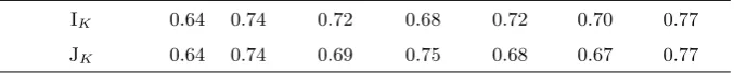
Shrinkage on Lags SP SMALL MEDIUM LARGE VLARGE GIANT FACTORS
IK 0.64 0.74 0.72 0.68 0.72 0.70 0.77
JK 0.64 0.74 0.69 0.75 0.68 0.67 0.77
Table 2: The valuesR2
pseudofor givenλ(see Table 1).
Remember that λ is selected in such a way to achieve equal in-sample fit
of model SMALL in the first estimation period (corresponding roughly to the
half of the total observations available in the data). It is therefore normal
that the final R2
pseudo values are different when I consider the entire time span
[image:14.595.137.476.590.625.2]where I have IK and JK. Adding more variables to the model, when shrinking,
does not improve its fit. Notice, that I do not shrink the parameters of model
FACTORS and thus it seems to have the best in-sample fit.
It is interesting to see how the models would perform in terms of in-sample
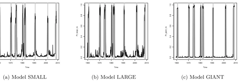
predictions if I do not impose any shrinkage (i.e. set λ large). In Figure 2, I
depict the results when all the models are estimated without applying any
shrinkage on the parameters.
Time
Pt_small
1960 1970 1980 1990 2000 2010
0.0 0.2 0.4 0.6 0.8 1.0
(a) Model SMALL
Time
Pt_large_ns
1960 1970 1980 1990 2000 2010
0.0 0.2 0.4 0.6 0.8 1.0
(b) Model LARGE
Time
Pt_giant_ns
1960 1970 1980 1990 2000 2010
0.0 0.2 0.4 0.6 0.8 1.0
[image:15.595.108.518.232.371.2](c) Model GIANT
Figure 2: In-sample fit without shrinkage.
The figures already indicate that in the absence of shrinkage, as expected,
larger models achieve very accurate in-sample fit. For example, in model
GIAN T the fitted values mimic the recession indicator almost perfectly. This
good in-sample performance can also be seen in theR2
pseudo-values reported
in Table 3.
SP SMALL MEDIUM LARGE VLARGE GIANT FACTORS
0.64 0.74 0.75 0.82 0.89 0.95 0.77
Table 3: The values of theR2
pseudo for the different models, withλ= 100.
As expected, imposing no shrinkage on the parameters leads to very good
in-sample fit, and it is monotonically increasing with the size of the model
as smaller models are just subsets of the largest model. However, we have
to bear in mind that good in-sample fit does not necessarily imply accurate
forecasting performance out of sample. Actually, due to overfitting, it is likely
that models with very high predictive accuracy in-sample may have very poor
forecasting performance. Out-of-sample forecasts are examined in more detail
4.3 Out-of-sample Results
I now turn to the out-of-sample forecasting performance of the models by
looking at the estimated posterior mean probabilities of recession computed
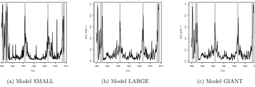
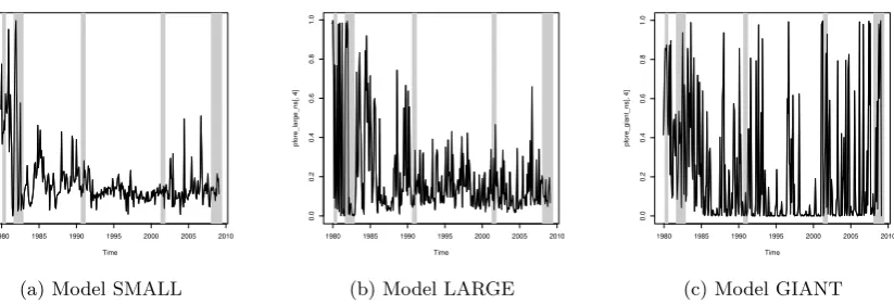
using (2.9) and (2.11). In Figure 3, I present the plots of the mean of the
posterior predictive distributions, our point estimates for the probability of
recession, one-month-ahead (h=1) using shrinkage method described above.
Time
pf
ore_small[, 1]
1980 1985 1990 1995 2000 2005 2010
0.0
0.2
0.4
0.6
0.8
1.0
(a) Model SMALL
Time
pf
ore_large[, 1]
1980 1985 1990 1995 2000 2005 2010
0.0
0.2
0.4
0.6
0.8
1.0
(b) Model LARGE
Time
pf
ore_giant[, 1]
1980 1985 1990 1995 2000 2005 2010
0.0
0.2
0.4
0.6
0.8
1.0
[image:16.595.102.512.221.361.2](c) Model GIANT
Figure 3: One-month-ahead forecasts with shrinkage.
The plots in Figure 3 already indicate that the shrinkage strategy works
well in forecasting recessions in the near future. Model GIANT, which has
more than 100 predictors, seems to provide pretty accurate one-month-ahead
forecasts without producing any false alarm. An example of a false alarm is
visible in the model SMALL around the year 2006, where the probability of
recession in the next month reaches 0.7, but as we can see that there was no
recession around that time.
While interesting from a methodological perspective, and in a possible
nowcasting setting, forecasting recessions one-month-ahead have not been the
main focus of the literature. Studies as Chauvet and Potter (2005) and Nyberg
(2010), among others, have focused on long-horizon recession forecasting, most
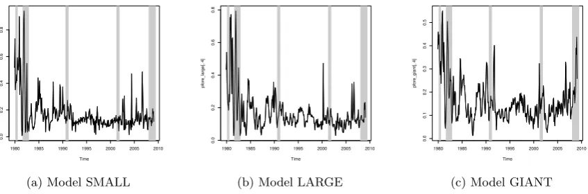
commonly one-year-ahead. Therefore, in Figure 4 I report the plots for the
Time
pf
ore_small[, 4]
1980 1985 1990 1995 2000 2005 2010
0.0
0.2
0.4
0.6
0.8
(a) Model SMALL
Time
pf
ore_large[, 4]
1980 1985 1990 1995 2000 2005 2010
0.0
0.2
0.4
0.6
0.8
(b) Model LARGE
Time
pf
ore_giant[, 4]
1980 1985 1990 1995 2000 2005 2010
0.0 0.1 0.2 0.3 0.4 0.5
[image:17.595.94.518.82.222.2](c) Model GIANT
Figure 4: 12-month-ahead forecasts with shrinkage.
There are few things we need to be aware of, when examining these plots.
It seems that larger models provide much less volatile forecasts compared with
the model including only five variables (SMALL) and no shrinkage. While
one-year-ahead recession forecasts in model GIANT never reach very high
recession probabilities, it is pretty clear when the recession probability spikes
with respect to non-recession periods. This result is line with the findings of
Kauppi and Saikkonen (2008), where dynamic models seem to give weaker,
albeit sharper signals of actual recessions in contrast of slowdowns of the
economy during expansions. Moreover, it seems that model GIANT is able
to forecast the recessions, without creating too many false alarms. Actually,
most of the false alarms produced by the model GIANT are in proximity of
the recession periods so they provide important information regarding the
future state of the economy. Only around the year 1983, the model GIANT
create a false alarm which is far from the subsequent recession. On the other
hand, more parsimonious models such as SMALL and LARGE have difficulties
in forecasting the early 1990s and 2000s recessions, together with the latest
(2008-2009) recession. However, these two models do a good job in forecasting
the recessions in the 80’s.
Figure 3 and 4 are useful to get a grasp of the forecasting performance
of our models but numerical indicators are easier to interpret in comparing
the predictive accuracy of the models under examination. Below, in Table
4, I report the QPS-statistics (4.1), for the models described in Section 3 for
forecast horizons h = 1,6,9 and 12 , where λ is set according to Table 1. I
we use the matrix IK) and with smaller λ imposed on the higher order lags
(matrix JK).
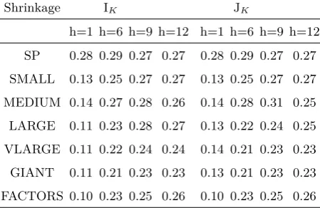
Shrinkage IK JK
h=1 h=6 h=9 h=12 h=1 h=6 h=9 h=12
SP 0.28 0.29 0.27 0.27 0.28 0.29 0.27 0.27
SMALL 0.13 0.25 0.27 0.27 0.13 0.25 0.27 0.27
MEDIUM 0.14 0.27 0.28 0.26 0.14 0.28 0.31 0.25
LARGE 0.11 0.23 0.28 0.27 0.13 0.22 0.24 0.25
VLARGE 0.11 0.22 0.24 0.24 0.14 0.21 0.23 0.23
GIANT 0.11 0.21 0.23 0.23 0.13 0.21 0.23 0.23
[image:18.595.192.417.121.267.2]FACTORS 0.10 0.23 0.25 0.26 0.10 0.23 0.25 0.26
Table 4: Out-of-sample QPS statistics for the models with shrinkage and matrix IK and JK.
It is clear that adding real activity predictors (going from SP to SMALL)
improves considerably short-term forecasts while it does not seem to have
a large effect on the longer term horizons. This result is likely to reflect
the presence of information (as discussed in Section 3) about the coincident
state of the economy at the time the forecast is computed. Even though the
determination of recession periods reflect a somewhat subjective judgment,
coincident indicators such as the ones included in SMALL and the larger
dataset are strongly correlated with the NBER’s definition of a recession.
However, the long-term forecasts are largely unaffected by the inclusion of
real economic activity indicators. This is due to the fact that the term-spread
(already present in the simplest model) is a dominant leading indicator for
recession periods. Nevertheless, increasing the set of explanatory variables,
while shrinking the parameters toward zero, provides superior forecasting
performance at all the forecast horizons. Model GIANT creates the most
accurate forecasts between the specifications considered here. For example,
12-month-ahead forecasts obtained with model SP present 14% larger value of
the out-of-sample QPS than model GIANT. However, the model FACTORS
provides the best one-month-ahead forecasts.
As we can see in Table 4, imposing matrix JK, instead of the identity
matrix, to shrink the parameters of larger models does not seem to influence
a lot the out-of-sample performance. Only model LARGE seems to benefit
Finally, it is interesting to see how the models would perform in the case of
no-shrinkage. First, in Figures 5 and 6, I provide plots of the posterior mean
predictive distributions for the forecast horizons h = 1 andh = 12 with no
shrinkage.
Time
pf
ore_small[, 1]
1980 1985 1990 1995 2000 2005 2010
0.0 0.2 0.4 0.6 0.8 1.0
(a) Model SMALL
Time
pf
ore_large_ns[, 1]
1980 1985 1990 1995 2000 2005 2010
0.0 0.2 0.4 0.6 0.8 1.0
(b) Model LARGE
Time
pf
ore_giant_ns[, 1]
1980 1985 1990 1995 2000 2005 2010
0.0 0.2 0.4 0.6 0.8 1.0
[image:19.595.104.516.169.310.2](c) Model GIANT
Figure 5: 1-month-ahead forecasts with no shrinkage.
Time
pf
ore_small[, 4]
1980 1985 1990 1995 2000 2005 2010
0.0
0.2
0.4
0.6
0.8
(a) Model SMALL
Time
pf
ore_large_ns[, 4]
1980 1985 1990 1995 2000 2005 2010
0.0 0.2 0.4 0.6 0.8 1.0
(b) Model LARGE
Time
pf
ore_giant_ns[, 4]
1980 1985 1990 1995 2000 2005 2010
0.0 0.2 0.4 0.6 0.8 1.0
(c) Model GIANT
Figure 6: 12-month-ahead forecasts with no shrinkage.
As expected, the forecasting performance seems to deteriorate greatly
when I do not impose any shrinkage on larger models. The forecasts become
extremely volatile at both long and short-term horizons, creating many false
alarms and giving no useful information to policy makers. To confirm these
findings, in Table 5, I present the QPS statistics for the forecasting models
[image:19.595.104.516.364.504.2]Model h=1 h=6 h=9 h=12
SP 0.23 0.26 0.26 0.26
SMALL 0.13 0.23 0.27 0.25
MEDIUM 0.20 0.30 0.32 0.31
LARGE 0.13 0.32 0.31 0.33
VLARGE 0.16 0.34 0.36 0.35
GIANT 0.17 0.35 0.32 0.33
FACTORS 0.10 0.23 0.25 0.26
Table 5: QPS for the models with no shrinkage.
We see that imposing a flat prior deteriorates the forecasting performance
of larger models substantially. This confirms the need of shrinkage when
increasing the set of explanatory variables. This is expected as the models
with a large number of predictors suffer from overfitting.
Looking at the empirical results gathered in this section, it seems that
model GIANT generally provides the best out-of-sample performance, at
least for forecast horizons longer than one month. Moreover, as we saw in
Figure 4, model GIANT provides useful insights to predict the state of the
economy when going beyond the actual QPS values. While the computed
recession probabilities never reach high values, the spikes during the economic
downturns are clearly visible. The good performance of large models is a
remarkable result also in the light of actual implementability. Nowadays,
large datasets are available to central banks, statistical offices and many other
institutions, so being able to use all the information available to forecast the
future state of the economy is highly beneficial. Bayesian shrinkage examined
in this paper allows us to deal with large information set without incurring
into the problem of overfitting and, as we have seen above, giving competitive
out-of-sample forecasts.
5
Conclusions
The use of large datasets in macroeconomic forecasting has been widely
adopted in the last few decades. However, in forecasting business cycle
recession periods, the literature has focused on the use of a small number of
into the analysis have relied on the use of factor-based models (see, e.g.,
Christiansen et al. (2014)), where the extracted factors are employed in the
probit model. In this study, I adopt a Bayesian shrinkage approach to estimate
probit models which include a large number of predictive variables. I set the
shrinkage proportionally to the number of predictors included so that the
(in-sample) predictive power of larger models is equal to the specification with
only a handful of predictors. In terms of the in-sample fit, the methodology
works well, preventing overfitting issues even for the models with more than
100 predictors. The ability of using a large number of predictors, without
estimating latent factors is the key contribution of this research. Bayesian
shrinkage facilitates economic interpretation of the predictors in the analysis
(contrary to factor-model based forecasts, which rely on extracted common
components with no clear economic interpretation).
I find that the probit model including all the predictive variables yields the
best out-of-sample predictions for all forecast horizons. Models including a
large number of predictors are able to beat the factor-based model, albeit the
latter gives us the best one-month-ahead forecasts. Moreover, the forecasts
from the largest model, even for the 12-month horizon, do not present evident
false alarms, while they provide a clear indication of when future recession
is likely. This result holds true for all the recession periods we have in our
sample.
The models we have considered here are static, i.e. they do not include
any dynamics of the recession indicator or the latent variable underlying
it. While the presence of large information sets, especially the inclusion of
coincident indicators such as industrial production, should already compensate
for missing dynamics, it could be interesting to examine in the future research
(outside the scope of this paper) dynamic models similar to Chauvet and
Potter (2005). Another interesting extension of this paper lies in the priors’
selection. In this study, I shrink all the parameters toward 0. However, we
know from previous literature that a subset of predictors are especially useful
in recession forecasting. It could be beneficial to impose priors that reflect
this knowledge, i.e. shrinking toward non-zero values, possibly drawn from
to include large amount of variables is desirable in a real-time environment,
where the decision makers might have access to large data, but do not have
a clear guidance on which variables to select. Examining the forecasting
performance of our models in a real-time analysis, where we take into account
the time delays due to the publication lags of different variables including the
binary recession indicator, can also be the subject of future research.
References
James H. Albert and Siddhartha Chib. Bayesian analysis of binary and
poly-chotomous response data. Journal of the American Statistical Association,
88(422):pp. 669–679, 1993.
Jushuan Bai and Serena Ng. Determining the Number of Factors in
Approxi-mate Factor Models. Econometrica, 70(1):191–221, 2002.
Marta Banbura, Domenico Giannone, and Lucrezia Reichlin. Large Bayesian
Vector Auto Regressions. Journal of Applied Econometrics, 25(1):71–92,
2010.
Marcelle Chauvet and Simon Potter. Forecasting recessions using the yield
curve. Journal of Forecasting, 24(2):77–103, 2005.
Zhihong Chen, Azharand Iqbal, and Huiwen Lai. Forecasting the probability of
US recessions: a Probit and dynamic factor modelling approach. Canadian
Journal of Economics, 44(2):651–672, 2011.
Charlotte Christiansen, Jonas N. Eriksen, and Stig V. Møller. Forecasting
US recessions: The role of sentiment. Journal of Banking and Finance, 49
(C):459–468, 2014.
Christine De Mol, Domenico Giannone, and Lucrezia Reichlin. Forecasting
using a large number of predictors: Is Bayesian shrinkage a valid alternative
to principal components? Journal of Econometrics, 146(2):318–328, 2008.
Michael Dueker. Strengthening the case for the yield curve as a predictor of
Arturo Estrella. A New Measure of Fit for Equations with Dichotomous
Dependent Variables. Journal of Business and Economic Statistics, 16(2):
198–205, 1998.
Arturo Estrella and Frederic S. Mishkin. Predicting U.S. Recessions: Financial
Variables As Leading Indicators. Review of Economics and Statistics, 80(1):
45–61, 1998.
Sebastian Fossati. Forecasting U.S. Recessions with Macro Factors. Working
Papers 2013-3, University of Alberta, Department of Economics, 2013.
Heikki Kauppi and Pentti Saikkonen. Predicting U.S. Recessions with Dynamic
Binary Response Models.Review of Economics and Statistics, 90(4):777–791,
2008.
Massimiliano Marcellino, James H. Stock, and Mark W. Watson. A comparison
of direct and iterated multistep AR methods for forecasting macroeconomic
time series. Journal of Econometrics, 135(1-2):499–526, 2006.
Henri Nyberg. Dynamic probit models and financial variables in recession
forecasting. Journal of Forecasting, 29(1-2):215–230, 2010.
Henri Nyberg. A bivariate autoregressive probit model: Business cycle linkages
and transmission of recession probabilities. Macroeconomic Dynamics, 18:
838–862, 2014.
Richard Startz. Binomial Autoregressive Moving Average Models With an
Application to U.S. Recessions. Journal of Business and Economic Statistics,
26:1–8, 2008.
James H. Stock and Mark W. Watson. Macroeconomic forecasting using
diffusion indexes.Journal of Business and Economic Statistics, 20(2):147–62,
2002.
James H. Stock and Mark W. Watson. Generalized Shrinkage Methods for
Forecasting Using Many Predictors. Journal of Business and Economic
Statistics, 30(4):481–493, 2012.
Jonathan H. Wright. The yield curve and predicting recessions. Finance and
Economics Discussion Series 2006-07, Board of Governors of the Federal
A. Zellner. An Introduction to Bayesian Inference in Econometrics. Wiley