Nowcasting and forecasting US recessions: Evidence from the Super Learner

(1)

Munich Personal RePEc Archive

Nowcasting and forecasting US

recessions: Evidence from the Super

Learner

Maas, Benedikt

Hamburg University

September 2019

Online at

https://mpra.ub.uni-muenchen.de/96408/

(2)

Nowcasting and forecasting US recessions:

Evidence from the Super Learner

Benedikt Maas

*

September 2019

Abstract

This paper introduces the Super Learner to nowcast and forecast the probability of a US econ-omy recession in the current quarter and future quarters. The Super Learner is an algorithm that selects an optimal weighted average from several machine learning algorithms. In this paper, elastic net, random forests, gradient boosting machines and kernel support vector machines are used as underlying base learners of the Super Learner, which is trained with real-time vintages of the FRED-MD database as input data. The Super Learner’s ability to categorise future time periods into recessions versus expansions is compared with eight different alternatives based on probit models. The relative model performance is evaluated based on receiver operating charac-teristic (ROC) curves. In summary, the Super Learner predicts a recession very reliably across all forecast horizons, although it is defeated by different individual benchmark models on each horizon.

JEL classification: C32, C53, C55, E32

*_{Hamburg University, Department of Economics, Von-Melle-Park 5, 20146 Hamburg, Germany; E-mail:}

(3)

1. Introduction

Accurately predicting turning points in the economy and identifying recessions is of great im-portance for economic agents, such as central bankers and policy makers. Previous research has shown that probit models and related approaches are powerful and reliable tools to clas-sify recessions (see Estrella and Hardouvelis (1991), Estrella and Mishkin (1996), Estrella and Mishkin (1998), Stock and Watson (1989), and Liu and Moench (2016)). However, these ap-proaches can only use a limited amount of forward-looking predictor variables. In contrast, machine learning algorithms are able to cope with a huge set of data and they can capture any non-linearities in the data.

A key question in the application of machine learning algorithms is the selection of the most predictive algorithm. However, there is still no consensus in the economic literature on which machine learning algorithm is most promising in detecting recessions. Against the backdrop of the Great Recession 2008/09, researchers have used different machine learning methods to predict recessions. For example, Ng (2014) and Döpke et al. (2017) use boosted regression trees (BRTs), whereas Gogas et al. (2015) use support vector machines (SVMs). By acknowledging that different algorithms have different advantages under certain circumstances, this paper takes an alternative path and develops a methodology that uses an ensemble of different algorithms to combine the best properties of each machine learning method. This ensemble learner is the so called “Super Learner” of van der Laan et al. (2007), which is an algorithm that selects an optimal weighted average of multiple machine learning algorithms. Jung et al. (2018) have been the first using the Super Learner for forecasting GDP growth, while this paper introduces the Super Learner as a tool for nowcasting and forecasting the likelihood of a US recession in the current quarter and in the following four quarters. The Super Learner is built from four widely-used machine learning algorithms, namely elastic net, random forests, gradient boosting machines (GBMs) and kernel support vector machines (KSVMs). These specific algorithms are chosen as so called “base learners” because they are the most commonly used classification tools in the machine learning literature.

(4)

conducted after the second month of each quarter, where the Super Learner algorithm is trained with a large database on past values of the National Bureau of Economic Research (NBER) recession indicator.

The Super Learner’s performance is compared with a total of eight benchmark models, which are all based on standard univariate and multivariate probit models. Four benchmark models are based on nowcast and forecast values of US GDP growth which are then used as predictor vari-ables in the probit models. The nowcasts and forecasts of the GDP growth values are obtained from: i) a multilayer perceptron (MLP), ii) an extreme learning machine (ELM), iii) a dynamic factor model (DFM), and iv) the Survey of Professional Forecasters (SPF). Several studies have shown the predictive power of the term structure of Treasury yields to forecast recessions (Es-trella and Hardouvelis, 1991; Es(Es-trella and Mishkin, 1998). Recently, Liu and Moench (2016) show that at short forecast horizons, adding a few leading financial and economic indicators can improve the recession predictability relative to forecasts based only on the Treasury term spread and its lags. Following their study, the remaining benchmark models are based on the term spread and its lagged value, which are combined with different economic and financial covariates: i) all nonfarm payroll employees, ii) returns on the S&P 500 common stock price index, iii) the spread between the yield of one-year constant maturity Treasuries and the federal funds rate, and iv) the spread between the yield of five-year constant maturity Treasuries and the federal funds rate.

Finally, the ability of the individual models to categorise current and future periods in reces-sions versus expanreces-sions is measured by receiver operating characteristic (ROC) curves and the corresponding area under receiver operating characteristic (AUROC) curves, as in Jordà and Taylor (2011) and Jordà and Taylor (2012). In summary, the Super Learner predicts a recession very reliably across all forecast horizons, although it is defeated by different benchmark models on each horizon.

The remainder of this paper is organised as follows. Section 2 introduces the Super Learner algorithm, the four different machine learning algorithms of the Super Learner, the benchmark models and the model evaluation procedure. Section 3 describes the applied data. Section 4 presents the empirical results. Finally, Section 5 concludes.

2. Methodology

(5)

ran-dom forests, GBMs and KSVMs are used as underlying base learners in this paper. These four machine learning algorithms are selected because they are considered to be the most common classification models within the machine learning literature. Furthermore, the benchmark mod-els are presented, which are based on standard probit modmod-els with different predictor variables. Finally, the model evaluation measures—ROC curve and AUROC—are described.

2.1. Super Learner

The Super Learner is an algorithm that selects an optimal weighted average of multiple machine learning algorithms. It was first introduced in van der Laan et al. (2007) and Dudoit and van der Laan (2005), and is a generalisation of the stacking algorithm introduced by Wolpert (1992),

which was adopted to model linear regressions by Breiman (1996b).1 _{This algorithm can be}

used for both regression applications or classification problems, and it can handle large datasets. In the context of prediction, the Super Learner algorithm applies a set of candidate predic-tion algorithms— the base learners—to the underlying dataset. The base learners can be any parametric or nonparametric supervised machine learning algorithm and the Super Learner the-ory does not require any specific level of diversity among the set of base learners. The Super Learner then works as a “metalearner” to find the optimal combination of the set of base learn-ers. The metalearner algorithm is typically a method designed to minimise the cross-validated risk of some loss function—for example the mean squared prediction error. Because the set of predictions from the different base learners may be highly correlated, it is advisable to choose a metalearning method like the Super Learner which performs well in the presence of collinear predictions (Bühlmann et al., 2016).

In the following, the general Super Learner algorithm for prediction is described. The de-scription that follows is based on Polley and van der Laan (2010) and van der Laan et al. (2007). Suppose the learning datasetXi= (Yi,Wi)fori=1, . . . ,n, whereY is the outcome of interest

and W is a p-dimensional set of covariates. The objective is to estimate the function ψ0 =

E(Y|W). The function can be expressed as the minimiser of the expected loss:

ψ0(W) =arg min

ψ E[L(X,ψ(W))], (2.1)

where the loss function is often the squared error loss:L2:(Y−ψ(W))2. For a given problem,

a “library” of various different prediction algorithms can be proposed. Denote the library as L

and the cardinality ofLasK(n).

1_{Wolpert (1992) and Breiman (1996b) used the same underlying algorithm with different tuning parameters as}

(6)

1. Fit each algorithm inLon the entire datasetX={Xi:i=1, . . . ,n}to estimateΨbk(W), k=

1, . . . ,K(n).

2. Split the dataset X into training and validation sample, according to a V-fold

cross-validation scheme: split the orderednobservations intoV-equal size groups, let thev-th

group be the validation sample, and the remaining group the training sample,v=1, . . . ,V.

DefineT(v)to be thevth training data split andV(v)to be the corresponding validation data split.T(v) =X\V(v), v=1, . . . ,V.

3. For thevth fold, fit each algorithm in Lon T(v) and save the predictions on the

corre-sponding validation data,Ψb_k_,_T₍_v₎(Wi), Xi∈V(v)forv=1, . . . ,V.

4. Stack the predictions from each algorithm together to create anbyK matrix,

Z=nΨb_k_,_T₍_v₎ W_V₍_v₎, v=1, . . . ,V and k=1, . . . ,Ko, where the notation

W_V₍_v₎= (Wi:Xi∈V(v))is used for the covariate-vectors of theV(v)-validation sample.

5. Propose a family of weighted combinations of the candidate estimators indexed by weight-vectorα:

m(z|α) =

K

∑

k=1

αkΨbk,T(v) WV(v)

, αk≥0 ∀k, K

∑

k=1

αk=1. (2.2)

6. Determine theα that minimises the cross-validated risk of the candidate estimator

∑K_k₌₁α_kΨb_kover all allowedα-combinations:

b

α =arg min

α

n

∑

i=1

(Yi−m(zi|α))2. (2.3)

7. Combineα_bwithΨb_k(W), k=1, . . . ,K according to the familym(z|α)of weighted

com-binations to create the final Super Learner fit:

b

Ψ_SL(W) =

K

∑

k=1b

αkΨbk(W). (2.4)

Theoretical results show that such an optimal learner will perform asymptotically as well as or better than any of the candidate base learners (van der Laan et al., 2007). This motivated the naming “Super Learner” since it provides a system of combining many estimators into an improved estimator (Polley and van der Laan, 2010).

(7)

2.1.1. Elastic net

The first base learner to be presented is the elastic net. The elastic net algorithm was origi-nally proposed by Zou and Hastie (2005) and is a combination of the ridge and least absolute shrinkage and selection operator (LASSO) regressions. Both approaches are forms of penalised regressions which generally improves ordinary least squares (OLS) regressions by using di-mension reduction and variable selection approaches when dealing with large datasets. In the following, the ridge and LASSO regressions are both briefly stated, before the elastic net is presented. The description that follows is based on Tiffin (2016) and Jung et al. (2018).

In general, the ridge regression minimises the residual sum of squares (RSS) and also an addi-tional shrinkage penalty term which decreases when the estimated coefficients of the regression become close to zero. When both the RSS and the shrinkage penalty are minimised, the optimal result will be achieved by shrinking those regressors of the dataset which are correlated. The overall minimisation problem is given as follows:

b

β =arg min

b βj       n

∑

i=1

Y−Xβb2

| {z }

RSS

+λ

p

∑

j=1

b

βj

2

| {z }

ridge penalty     

, (2.5)

wherenis the number of observations, pthe number of explanatory variables andλ denotes the

shrinkage penalty parameter, which will be determined by iterative cross-validation. A higher

λ will lead to a stronger shrinkage, whereas a λ of zero produces the same result as standard

OLS regression.

The LASSO was proposed by Tibshirani (1996) and also shrinks the coefficients of an OLS regression, but uses a different penalty term compared to the ridge regression. The overall minimisation problem is then given as follows:

b

β =arg min

b βj       n

∑

i=1

Y−Xβb2

| {z }

RSS

+ λ

p

∑

j=1

bβj

| {z }

LASSO penalty      . (2.6)

In Equation (2.6), zero coefficients are possible if the parameter λ is large enough. Hence,

(8)

Finally, the elastic net algorithm combines both penalty terms from Equations (2.5) and (2.6):

b

β =arg min

b βj      n

∑

i=1

Y−Xβb2

| {z }

RSS

+λ

p

∑

j=1

  

(1−α)

b

βj

2

| {z }

ridge

+α_bβj

| {z }

LASSO        

, (2.7)

where the parameter α determines the relative weights of the penalty terms. It is selected via

cross-validation. In general, the elastic net combines the advantages from both the ridge

regres-sion and the LASSO and overcomes their individual weakness.2 _{Zou and Hastie (2005) state}

that the elastic net is superior or at least as good as both standalone models in situations where the number of regressors exceed the number of observations (“fat data”), when the number of observations largely exceeds the number of regressors (“tall data”) or when multiple variables are highly correlated.

2.1.2. Random forests

Beside elastic net, the Super Learner algorithm can also choose random forests as potential base learner. In general, random forests belong to the family of decision trees. They were proposed by Breiman (2001) and they are an advancement of the related classification tree algorithm called bagging (bootstrap aggregating) introduced by Breiman (1996a). In bagging, the decision trees are not completely independent of each other since all variables are considered at every split of the tree. Random forests overcome this feature by adding an additional layer of randomness.

Similar to bagging, random forests also construct each tree using a different bootstrap sample of the data, but they change how the classification trees are constructed. In bagging, each node is split using the best split among all variables, whereas in random forests, each node is split using the best among a subset of variables randomly chosen at that node. This strategy turns out to perform very well compared to other classifiers and is also robust against overfitting (Breiman, 2001).

The description about the random forests algorithm that follows is based on Efron and Hastie (2016):

Suppose a training set consisting of ann×pdata matrixX and ann-vector of responsesy.

1. Given the training datasetd= (X,y), fixm≤ pand the number of treesB.

2_{For extensive details about the ridge regression, the LASSO and the elastic net, see Zou and Hastie (2005) and}

(9)

2. Forb=1,2, . . . ,Bdo the following:

a) Create a bootstrap version of the training datad_b∗, by randomly sampling thenrows

with replacementntimes.

b) Grow a maximal-depth tree_brb(x)using the data indb∗, samplingmof the pfeatures

at random prior to making each split.

c) Save the tree, as well as the bootstrap sampling frequencies for each of the training observations.

3. Compute the random forests fit at any prediction pointx0as the average

brr f(x0) =

1

B

∑

b=1b

rb(x0). (2.8)

4. Compute the “out-of-bag” error OOBi for each response observation yi in the training

data, by using the fit_br_{r f}(i), obtained by averaging only those_brb(xi)for which observationi

was not in the bootstrap sample. The overall OOB error is the average of these OOBi.

2.1.3. Gradient boosting machine

GBMs are based on multiple decision trees like random forests, but the treatment of the single trees is rather different. In general, the term “boosting” has been originally developed for clas-sification problems. The first boosting algorithms were introduced by Schapire (1990), Freund (1995) and Freund and Schapire (1999) and they combine (or “boost”) a number of weak classi-fiers (a classifier that predicts marginally better than random) into a superior ensemble classifier. One of the most popular boosting algorithm is the Adaboost (“Adaptive boosting”) algorithm (Freund and Schapire, 1997), which was then connected by Friedman et al. (2000) to statistical concepts of loss functions and logistic regressions, showing that boosting can be interpreted as a forward stagewise additive model that minimises exponential loss.

Friedman (2001) developed a highly adaptable method for both classification and regression problems which he called “gradient boosting machine”. The intuition of Friedman’s GBMs taken from Kuhn and Johnson (2013) is the following:

(10)

number of iterations. When trees are used as the base learner, basic gradient boosting machine

has three tuning parameters: number of iterationsB, tree depthd, and shrinkage parameterε.

A more formal presentation of the gradient boosting machine is briefly stated in the following. The notation is based on Efron and Hastie (2016). Suppose that we are interested in modeling

µ(x) =Pr(Y =1|X =x) for a Bernoulli response variable. The idea is to fit a model of the

form

λ(x) =GB(x) =

B

∑

b=1

gb(x;yb), (2.9)

whereλ(x)is the natural parameter in the conditional distribution ofY|X=x, andgb(x;yb)are

functions like shallow trees. In the case of the Bernoulli response, we have

λ(X) =log

_Pr

(Y =1|X =x)

Pr(Y =0|X =x)

. (2.10)

The gradient boosting algorithm works as follows:

1. Start withGb0(x) =0, and setBand the shrinkage parameterε >0.

2. Forb=1,2, . . . ,Brepeat the following steps:

a) Compute the pointwise negative gradient of the loss function at the current fit:

ri=−

∂L(yi,λi)

∂ λi

_λ

i=Gbb−l(xi)

, l=1, . . . ,n. (2.11)

b) Approximate the negative gradient by a depth-d tree by solving

min

y n

∑

i=1

(ri−g(xi;y))2. (2.12)

c) UpdateGbb(x) =Gbb−1(x) +gbb(x), withgbb=ε×g(x;byb).

3. Return the sequenceGbb(x),b=1, . . . ,B.

2.1.4. Kernel support vector machine

(11)

which divides the space to create partitions on either side. SVMs are most easily understood when used for binary classification within a linear framework, which is how the method has been traditionally applied.

However, in many real-world applications, the relationships between variables are non-linear. Nevertheless, SVMs can still be trained on non-linear data through the addition of a so-called “slack” variable, which to some extent allows for misclassification, or more promisingly by

the use of the so-called “kernel trick”, leading to KSVMs.3 The following brief explanation of

KSVMs is based on Kecman (2005):

Consider the problem of binary classification, where the training data are given as

(x1,y1),(x2,y2), . . . ,(xl,yl), x∈Rn, y∈ {+1,−1}. (2.13)

In the case of the classification of linearly separable data, the goal of a SVM is to find among all the hyperplanes that minimise the training error to find the one with the largest margin. This

is done by—using the given training examples—finding parametersw= [w1,w2, . . . ,wn]T and

the scalarbof the following decision functiond(x,w,b)

d(x,w,b) =wTx+b=

n

∑

i=1

wixi+b, (2.14)

where x,w∈Rn. After obtaining the weights, testing on unseen data xp the vector machine

produces output 0 according to an indicator function given as

iF =o=sign(d(xp,w,b)), (2.15)

where ostands for output. The decision rule of the binary classification task is as follows: if

d(xp,w,b)>0, thenxpbelongs to class 1(o=y1= +1), and ifd(xp,w,b)<0, thenxpbelongs

to class 2(o=y2=−1).4

The intuition of the SVM works also for non-linear data, because KSVMs are able to map a problem into a higher dimension space using the kernel trick, making a non-linear relationship appear to be quite linear. The basic idea in designing non-linear KSVMs is to map input vectors

x∈Rninto vectorsΦ(x)of a higher dimensional feature spaceF (whereΦrepresents mapping:

Rn→Rf), and to solve a linear classification problem in this feature space

x∈Rn→Φ(x) = [φ1(x),φ2(x), . . . ,φn(x)]T ∈Rf. (2.16)

3_{For the kernel trick, see Schölkopf et al. (2002).}

(12)

The mappingΦ(x)is chosen in advance. By performing a mapping, in aΦ-space, the learning

algorithm will be able to linearly separate images ofxby applying the linear SVM framework.

This approach also leads to an optimisation problem with similar constraints in aΦ-space. The

solution for an indicator functioniF(x) =sign wTΦ(x) +b=sign ∑_il₌₁yiαiΦT(xi)Φ(x) +b,

which is a linear classifier in a feature space, creates a non-linear separating hypersurface in the original space by the following indicator function:

iF =sign l

∑

i=1

yiαiΦT(xi)Φ(x) +b

!

=sign

l

∑

i=1

yiαik(xi,x) +b

!

=sign

l

∑

i=1

vik(xi,x) +b

!

,

(2.17)

where vi corresponds to the output layer weights of the SVM and k(xi,x) denotes the value

of the kernel function. The kernel function is a function in input space. Thus, by using a

kernel function, it is no longer necessary to know the mapping Φ(x). Instead, the required

scalar products in a feature space ΦT₍_x

i)Φ xj are calculated directly by computing kernels

for given training data vectors in an input space. By using kernels, a KSVM can be constructed that operates in an infinite dimensional space and the extremely high dimensionality of a feature

spaceF is avoided. In general, a kernel is a functionKsuch that

K xi,xj

=ΦT(xi)Φ xj

. (2.18)

However, there are many different kernels to choose from and, therefore, this paper uses the Gaussian radial basis function kernel of the following form:

K(x,xi) =e 1

2[(x−xi)T∑−1(x−xi)]_, (2.19)

which is a general purpose kernel and is typically chosen when no prior knowledge is available about the data.

2.2. Benchmark models

(13)

univariate and multivariate probit models of the following form:

Pr(Yt+h=1|Xt =xi,t) =Φ β0+ k

∑

i=1 βixi,t

!

, (2.20)

where the dependent variable Y_t₊_h is the binary NBER recession indicator, h is the forecast

horizon,Φis the cumulative standard normal distribution function, andxi,t are up tokpredictor

variables.

The predictor variables are different across all the benchmark models. In four of the bench-mark models, the predictor variables are nowcasts and forecasts of GDP growth. These now-casts and forenow-casts are generated by two machine learning methods—to be precise a MLP and an ELM which are both types of artificial neural networks (ANNs)—by a standard DFM and taken from the SPF. Based on the research by Liu and Moench (2016), the remaining four benchmark models are multivariate probit models, where the term spread and its 6-month lag are combined with different economic and financial indicators as predictor variables. The term spread is defined in this paper as the difference between the ten-year and three-month Treasury yields.

A list of the benchmark probit models and a brief explanation of each approach is presented in the following:

1. Probit: MLP

Following the approach described in Loermann and Maas (2019), nowcasts and forecasts of GDP growth are first obtained by a MLP, which is a special kind of a feedforward ANN. This network is trained on a large database via the gradient-based learning algo-rithm called “backpropagation” (Rumelhart et al., 1986) and can be best interpreted as a flexible and highly parametrised non-linear autoregressive distributed lag model (ARDL)

model.5 The estimated GDP values then go into the univariate probit model as described

in Equation (2.20) to yield the recession probabilities for the different horizons.

2. Probit: ELM

The procedure is the same as under 1, but the feedforward ANN is an ELM based on Huang et al. (2006). In contrast to a MLP, an ELM does not use the slow gradient-based learning algorithm backpropagation to tune parameters of the hidden nodes. The output weights of the hidden nodes are randomly chosen and, therefore, are learned in a single step, so that the ELM learns faster as the MLP. The nowcasts and forecasts of GDP values

5_{For details about the MLP, see Crone and Kourentzes (2010), Kourentzes et al. (2014) and Lachtermacher and}

(14)

obtained from this ELM then go into the univariate probit model from Equation (2.20).

3. Probit: DFM

First, the GDP growth values for the current quarter and for future quarters are estimated from a large database of potential predictor variables by a DFM based on Giannone et al. (2008), as done in Loermann and Maas (2019). Then, the estimated values are used in the probit model to get the recession probabilities.

4. Probit: SPF

This benchmark model uses the nowcasts and forecasts of GDP growth published by the SPF, which are then used as predictor variables in the probit model. The Survey publishes

its nowcast and forecasts of future GDP growth around the mid of every quarter.6

5. Probit: term spread+Emp: total

This benchmark model is a multivariate probit model, where the predictor variables are the term spread, its 6-month lag and all nonfarm payroll employees.

6. Probit: term spread+S&P 500

Beside the term spread and its 6-month lag, returns on the S&P 500 common stock price index are included as covariate in the probit model.

7. Probit: term spread+1yr spread

In addition to the term spread and its 6-month lag, this benchmark includes as an ad-ditional variable in the probit model the spread between the yield of one-year constant maturity Treasuries and the federal funds rate.

8. Probit: term spread+5yr spread

The procedure is the same as under 7, but the spread between the yield of five-year con-stant maturity Treasuries and the federal funds rate is used as an additional covariate next to the term spread and its lagged value.

2.3. Evaluating the models

To measure which model has the best ability to nowcast and forecast recessions, the ROC curve and its corresponding AUROC value are used in this paper. The basic ROC methodology was

first introduced by Peterson et al. (1954), but has recently found its way into Economics.7

6_{For details about the SPF, see Croushore (1993).}

7_{For applications of the ROC in Economics, see for example Jordà and Taylor (2011, 2012), Khandani et al.}

(15)

The basic ROC methodology in the context of predicting recessions is summarised in the following, while the notation is adapted from Liu and Moench (2016):

1. Let

Zt =

(

1, if in recession

0, otherwise, (2.21)

denote the true, observed state of the economy. LetPt be the prediction ofZt—the

reces-sion probability—where 0≤Pt≤1.

2. Define evenly spaced thresholds, denoted asC∗, along the interval [0,1]. For example, a

set with 20 thresholds would beC∗={0,0.05, . . . ,0.95,1}.

3. For each given thresholdC∗_i, record the model’s predicted categories. Define the predicted

categorisationZbt as follows:

b

Zt =

(

1, if Pt ≥Ci∗

0, if Pt <Ci∗.

(2.22)

4. Comparing the trueZt with the predicted categorisationsZbt, calculate the percentages of

true positives (PTP) and the percentages of false positives (PFP).8 Both fractions can be

defined using the sum of two indicator variables:

PT Pi=

1

nR T

∑

t=1

I_tt p;

whereI_tt p=

(

1, if Zt=1 and Zbt=1

0, otherwise,

(2.23)

PFPi=

1

nE T

∑

t=1

I_tf p;

where I_tf p=

(

1, if Zt=0 and Zbt =1

0, otherwise,

(2.24)

where nR is the number of times the true Zt was in a recession and nE is the number

of times the true Zt was not in a recession, such that nR+nE =T, where T is the total

number of observations in the sample.

8_{In the empirical literature, the percentages of true positives (PTP) is also called ‘sensitivity’ and the percentages}

(16)

5. For eachC_i∗create a set of coordinates: (PFPi,PT Pi).

6. After a coordinate is created for each threshold, we plot the coordinates across all thresh-olds, with the false positive rate on the x-axis and the true positive rate on the y-axis. We then connect these coordinates to trace out the ROC curve.

In summary, a model with 100 % accuracy would have a ROC curve that covers the upper

left-hand corner. A model which is equivalent to a random guess would follow a 45◦ _diagonal

running from the bottom left-hand to the top right-hand corner.

Because it is visually very difficult to recognise which ROC curve gives the best overall predictive ability out of a set of different ROC curves, the curves are integrated and the resulting area under receiver operating characteristic (AUROC) curve is then compared. An AUROC value of one means that the model perfectly classifies a recession, where a value of 0.5 is equivalent to a random guess. In the empirical analysis in Section 4, the recession classification ability of the models will be compared by their implied AUROC values.

Given that the residuals from classification models that use a recession indicator as the de-pendent variable are likely to be autocorrelated, inference on the classification ability using the AUROC is given by the block bootstrap approach of Politis and Romano (1994), as done in Liu and Moench (2016) and Pierdzioch et al. (2018). The block bootstrap is implemented with 1000 simulation runs and—following Liu and Moench (2016)—a block length of eight years is used to retain the typical business cycle length. This procedure creates a comparable empirical distribution of AUROC values for each model and each forecast horizon.

3. Data

Before turning to the results, it is important to illustrate the data, particularly the challenges of real-time now- and forecasting.

(17)

Beginning with the introduction of the data, it can be noted that this study uses macroeco-nomic data as provided by the Federal Reserve Ecomacroeco-nomic Data (FRED) database. To be precise, the data behind the DFM, the MLP, the ELM and the Super Learner is the same and comes from FRED-MD, the monthly database for Macroeconomic Research of the Federal Reserve Bank of St. Louis, which is described extensively in McCracken and Ng (2016). The time series used in the remaining probit models are also retrieved from FRED but the nowcasts and forecasts of

the SPF are obtained from the Federal Reserve Bank of Philadelphia.9

In brief, FRED-MD is a large macroeconomic database that is designed for the empirical analysis of “big data”. The database is publicly available and updated in real-time on a monthly

basis.10 _{It consists of 134 monthly time series and is classified into eight categories: (1) output}

and income; (2) labor market; (3) housing; (4) consumption, orders and inventories; (5) money and credit; (6) interest and exchange rates; (7) prices; and (8) stock market. A full list of the data and its transformation is given in Appendix A.2. The time series start in January 1959 and vintages of the whole database are available since August 1999.

Before training the Super Learner, the time series contained in the vintage of the FRED-MD database are transformed to be stationary, outliers are removed, and missing values are replaced by the expectation-maximization (EM) algorithm; however, the ragged edge structure at the end of the sample is still unchanged. Because the NBER recession dates are quarterly, the monthly time series need to be transformed into quarterly equivalents. This paper follows Giannone

et al. (2008), who use a rational transfer function for this purpose.11 _{To deal with the ragged}

edge problem at the end of the sample, these missing values are filled up by applying univariate

ARMA(p;q)forecasts of each single time series, where the lag lengths are selected via Akaike

information criterion (AIC). This procedure is also done for the benchmark models. Then,

considering the training of the Super Learner, the data is scaled on the interval[0,1]and split

into five folds for cross-validation.

When it comes to training the Super Learner algorithm and estimating the probit models, the treatment of the NBER recession dates is of interest. Because the NBER Business Cycle Dating

Committee detects a recession with a certain delay12_{, all models are trained with a delay of four}

9_{The SPF can be downloaded from the following link:} _{https://www.philadelphiafed.org/}

research-and-data/real-time-center/survey-of-professional-forecasters/.

10_{The FRED-MD database is available for download under the following link:} _{https://research.}

stlouisfed.org/econ/mccracken/fred-databases/.

11_{Giannone et al. (2008) use the following rational transfer function to transform the data into a quarterly}

equiv-alent: Y(z) = b(1)+b(2)z−1+···+b(nb+1)z−nb

1+a(2)z−1₊_···₊_a₍_n_a₊₁₎_z−na X(z), with[a,b] = [1,(1,2,3,2,1)]. For further details, see the

Ap-pendix of Giannone et al. (2008).

12_{The NBER Business Cycle Dating Committee states that “there is no fixed timing rule” when it comes to a}

determination of a recession. “The committee waits long enough so that the existence of a peak or trough is

(18)

quarters before the final forecast is produced with the latest and most up-to-date data from the last update of the database. Furthermore, because the recession probability is to be predicted

for the current quarter and the following four quarters, the NBER recession date int is linked

to the predictor variables int−h, wherehstands for the horizonsh=0,1,2,3,4.

The nowcasts and forecasts of the recession probabilities are conducted at the end of the second month of each quarter. To allow the Super Learner and also the probit models to learn and adapt from new data, all models are retrained in the next period after an update of the respective input data.

4. Empirical results

This section presents the empirical results. The recession probabilities obtained from the Super Learner algorithm are compared with the results of the different probit models for the different forecast horizons using the respective AUROC value. The higher the AUROC, the better the ability to determine recessions, whereby the AUROC value cannot exceed a value of one. For each model, the standard errors obtained from the block bootstrap approach after Politis and Romano (1994) are also reported.

Due to data transformation and the lagged behavior of the NBER recession dates, the training sample of the first out-of-sample nowcasting and forecasting exercise starts in 1959Q3 and goes on until 1998Q2, which covers a total of six recessions after the NBER recession indicator. The first nowcast is then conducted for 1999Q3 and the first out-of-sample forecasts are made for the following four quarters. The last nowcast is made in 2019Q1. In addition, it is shown which machine learning methods the Super Learner is composed of at the individual points in time per prediction horizon.

In this empirical task, the Super Learner consists of a total of 1289 models per forecast horizon. The high number of different models results from a multitude of different tuning parameters with which the individual four machine learning methods are trained before making

the nowcasts and forecasts.13

Table 1 shows the empirical out-of-sample results. For horizonh=0—the nowcast—the SPF

reaches the highest AUROC value of 0.9937, followed by the Super Learner and the ‘Probit:

recessions_faq.htmlfor further information.

13_{As far as tuning parameters are concerned, random forests are trained with different number of trees} ₌

[100,150, . . . ,1000]. Gradient boosting machines are trained with number of trees= [100,200, . . . ,1000], depth

of the tree= [1,2, . . . ,10], shrinkage parameter= [0.001,0.005,0.01,0.1], and minimum observations allowed

per tree node= [1,3,5]. Kernel support vector machines are trained with the following tuning parameters:

(19)

DFM’-model, both with a value of 0.9810. All alternative models have a value above 0.94,

which highlights that they are all very successful in nowcasting a recession in the current quarter. When estimating the probability of a recession for future quarters, the AUROC value of

the Super Learner decreases. For horizonh=1, the Super Learner’s AUROC of 0.9614 is only

beaten by the ‘Probit: term spread+S&P 500’-model with a value of 0.9646. For horizonh=2,

the Super Learner is beaten by ‘Probit: term spread+Emp: total’, ‘Probit: term spread+S&P

500’, ‘Probit: term spread+1yr spread’, and ‘Probit: term spread+5yr spread’. For the longer

horizonsh=3 andh=4, the Super Learner clearly outperforms the MLP, the ELM, the DFM,

and the SPF, which highlights the limited power of these approaches for detecting recessions in the long-term. However, the Super Learner is considerably beaten by the probit models using the one-year Treasury spread and the five-year Treasury spread as additional predictors. The probit model with the five-year Treasury spread has the overall highest AUROC value for the

longer forecast horizonsh=2,h=3, andh=4, which illustrates the strong predictive power of

(20)

[image:20.595.77.524.94.384.2]

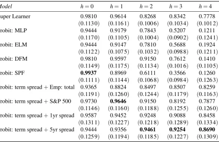
Table 1: Out-of-sample summary of AUROC values.

Model h=0 h=1 h=2 h=3 h=4

Super Learner 0.9810 0.9614 0.8268 0.8342 0.7778

(0.113 0) (0.116 1) (0.100 6) (0.103 4) (0.101 2)

Probit: MLP 0.9444 0.9179 0.7843 0.5207 0.1211

(0.117 0) (0.110 5) (0.100 4) (0.090 2) (0.124 1)

Probit: ELM 0.9444 0.9147 0.7810 0.5688 0.1924

(0.112 2) (0.107 5) (0.103 2) (0.098 8) (0.121 1)

Probit: DFM 0.9810 0.9597 0.9150 0.7612 0.1410

(0.114 9) (0.117 5) (0.113 4) (0.101 6) (0.110 5)

Probit: SPF 0.9937 0.8969 0.6111 0.3566 0.1260

(0.111 1) (0.114 4) (0.106 8) (0.098 4) (0.126 3)

Probit: term spread+Emp: total 0.9365 0.8824 0.8497 0.8507 0.8259

(0.119 1) (0.126 0) (0.124 4) (0.117 9) (0.116 3)

Probit: term spread+S&P 500 0.9730 0.9646 0.9150 0.8192 0.7877

(0.114 6) (0.116 0) (0.118 8) (0.125 5) (0.126 0)

Probit: term spread+1yr spread 0.9587 0.9452 0.9248 0.9088 0.8458

(0.131 1) (0.122 7) (0.121 8) (0.128 9) (0.133 4)

Probit: term spread+5yr spread 0.9444 0.9356 0.9461 0.9254 0.8690

(0.125 9) (0.119 4) (0.118 5) (0.122 7) (0.130 9)

Notes:This table shows the out-of-sample AUROC values for the sample period 1999Q3 - 2019Q1. The numbers in bold correspond to the

highest AUROC value at each forecast horizonh. The corresponding standard errors are reported in parentheses. Standard errors are computed

based on the bootstrapped sampling distribution of the AUROC statistic. The bootstrap was implemented through the block bootstrap approach of Politis and Romano (1994) with 1000 simulation runs and a block length of eight years.

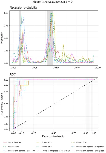
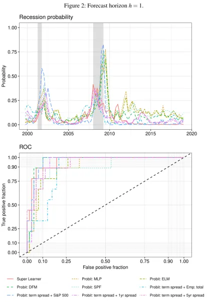
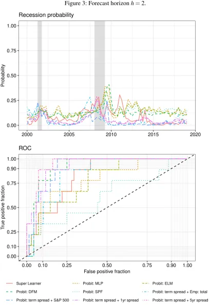
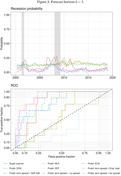
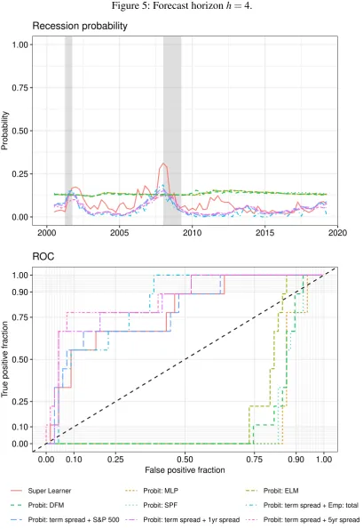
Figures 1-5 show the plotted recession probabilities and the corresponding ROC curves. All of the figures show that the Super Learner announces periods of economic turmoil in quite good time. In particular, it indicates an increased recession probability for all forecast horizons in the

run-up to the 2008/09 recession. Especially for the horizonsh=3 andh=4, the Super Learner

shows an increased recession probability in the period leading up to the Great Recession when compared to the benchmark models, highlighting the strength of its use of a larger dataset and different underlying powerful classification tools. However, the recession probability deter-mined for these horizons is more volatile than for the multivariate probit models, resulting in a lower AUROC value in each case.

It is of note that for the shorter forecast horizons h=0 and h=1, during the two NBER

recessions the recession probability determined by the Super Learner is lower than that of some benchmarks. Nevertheless, considering these horizons, the Super Learner seems best to an-nounce the approaching end of a recession because the probability of a recession decreases more strongly towards the end of each recession than most other benchmark models.

(21)

to predict recessions for the individual models with an increased forecast horizon because the ROC curves slide further and further in the direction of the lower right-hand corner, where at

horizon h=4 the ‘Probit: DFM’, ‘Probit: MLP’, ‘Probit: SPF’ and ‘Probit: ELM’ models

perform clearly worse than a random guess.

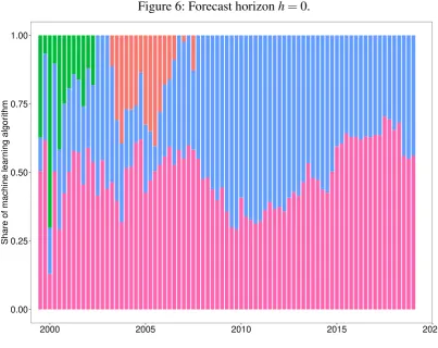
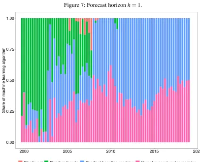
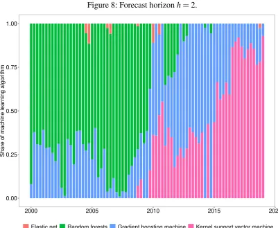
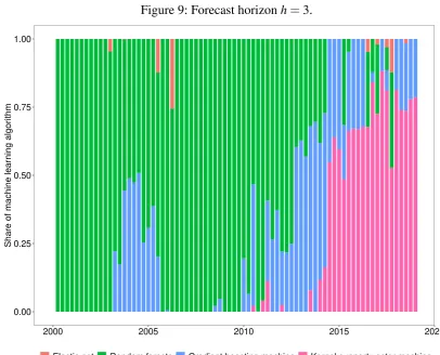
To gain further insight into which machine learning methods the Super Learner is composed of in each period—either elastic net, random forests, gradient boosting machines or kernel support vector machines—, the proportions of the four different methods are shown visually in

the Figures 6-10 in Appendix A.1 for each forecast horizon. It is of note that at horizonh=0

after 2008 the Super Learner consists only of gradient boosting machines and kernel support vector machines. Random forests are only used at the beginning of the sample and since 2004 elastic net has also been used. However, as the prediction horizon widens, the proportion of

random forests increases, especially at the beginning of each sample. At horizon h=4, this

(22)

[image:22.595.91.505.81.675.2]

Figure 1: Forecast horizonh=0.

0.00 0.25 0.50 0.75 1.00

2000 2005 2010 2015 2020

Probability

Recession probability

0.00 0.10 0.25 0.50 0.75 0.90 1.00

False positive fraction

T

rue positiv

e fr

action

ROC

Super Learner Probit: MLP Probit: ELM

Probit: DFM Probit: SPF Probit: term spread + Emp: total

Probit: term spread + S&P 500 Probit: term spread + 1yr spread Probit: term spread + 5yr spread

(23)

[image:23.595.90.504.76.680.2]

0.00 0.25 0.50 0.75 1.00

2000 2005 2010 2015 2020

Probability

0.00 0.10 0.25 0.50 0.75 0.90 1.00

T

rue positiv

e fr

action

ROC

(24)

[image:24.595.92.502.81.676.2]

0.00 0.25 0.50 0.75 1.00

2000 2005 2010 2015 2020

Probability

0.00 0.10 0.25 0.50 0.75 0.90 1.00

T

rue positiv

e fr

action

ROC

(25)

[image:25.595.92.502.81.676.2]

0.00 0.25 0.50 0.75 1.00

2000 2005 2010 2015 2020

Probability

0.00 0.10 0.25 0.50 0.75 0.90 1.00

T

rue positiv

e fr

action

ROC

(26)

[image:26.595.92.502.81.677.2]

0.00 0.25 0.50 0.75 1.00

2000 2005 2010 2015 2020

Probability

0.00 0.10 0.25 0.50 0.75 0.90 1.00

T

rue positiv

e fr

action

ROC

(27)

5. Conclusion

This paper applies the Super Learner algorithm to nowcast and forecast the probability of a re-cession in the US economy for the current quarter and for future quarters. The Super Learner is composed of four machine learning algorithms—namely, elastic net, random forests, gradient boosting machines and kernel support vector machines—and is trained with real-time vintages of the FRED-MD database. The obtained recession probabilities are compared with those of a total of eight benchmark models based on univariate and multivariate probit models. In four of the probit models, nowcasts and forecasts of GDP growth in the current quarter and the fol-lowing quarters are the only predictor variables, while in the remaining four the term spread, its 6-month lag and an additional economic or financial indicator variable are incorporated as additional predictors. To measure which model overall has the best ability to predict recessions across all horizons, this article uses the ROC curve and the corresponding AUROC. The now-casts and forenow-casts are conducted in real-time and are made at the end of the second month of each quarter.

In summary, the Super Learner presented in this paper can be described as a kind of all-rounder that can rely on large databases and which works well across all forecast horizons. When nowcasting a recession in the current quarter, all models are very successful in nowcast-ing a recession and the Super Learner is only beaten by the probit model with GDP nowcast published by the SPF as predictor variable. For the longer forecast horizons, the probit models including the term spread yield the highest AUROC values, where the model with the spread be-tween the yield of five-year constant maturity Treasuries and the federal funds rate as additional

predictor variable reaches the overall best results for horizonh=2,h=3, andh=4.

However, since the financial crisis of 2007/08, central banks have intervened significantly in the bond market through extensive asset purchase programmes and, therefore, the credibility and the forecasting ability of the yield curve can be questioned since that time. In contrast, the Super Learner algorithm used in this article is not affected by this problem because its predictions are based on the use of much larger and more diverse datasets.

(28)

References

Breiman, L. (1996a). Bagging predictors. Machine Learning, 24(2):123–140.

Breiman, L. (1996b). Stacked regressions. Machine Learning, 24(1):49–64.

Breiman, L. (2001). Random forests. Machine Learning, 45(1):5–32.

Bühlmann, P., Drineas, P., Kane, M., and van der Laan, M. J. (2016). Handbook of Big Data.

CRC Press.

Crone, S. F. and Kourentzes, N. (2010). Feature selection for time series prediction–a combined

filter and wrapper approach for neural networks. Neurocomputing, 73(10-12):1923–1936.

Croushore, D. D. (1993). Introducing: the Survey of Professional Forecasters.Business

Review-Federal Reserve Bank of Philadelphia, 6:3–15.

Döpke, J., Fritsche, U., and Pierdzioch, C. (2017). Predicting recessions with boosted regression

trees. International Journal of Forecasting, 33(4):745–759.

Dudoit, S. and van der Laan, M. J. (2005). Asymptotics of cross-validated risk estimation in

estimator selection and performance assessment. Statistical Methodology, 2(2):131–154.

Efron, B. and Hastie, T. (2016). Computer Age Statistical Inference, volume 5. Cambridge

University Press.

Estrella, A. and Hardouvelis, G. A. (1991). The term structure as a predictor of real economic

activity. The Journal of Finance, 46(2):555–576.

Estrella, A. and Mishkin, F. S. (1996). The yield curve as a predictor of US recessions. Current

Issues in Economics and Finance, 2(7).

Estrella, A. and Mishkin, F. S. (1998). Predicting US recessions: financial variables as leading

indicators. Review of Economics and Statistics, 80(1):45–61.

Freund, Y. (1995). Boosting a weak learning algorithm by majority. Information and

Compu-tation, 121(2):256–285.

Freund, Y. and Schapire, R. E. (1997). A decision-theoretic generalization of on-line learning

and an application to boosting. Journal of Computer and System Sciences, 55(1):119–139.

Freund, Y. and Schapire, R. E. (1999). Adaptive game playing using multiplicative weights.

(29)

Friedman, J., Hastie, T., and Tibshirani, R. (2010). Regularization paths for generalized linear

models via coordinate descent. Journal of Statistical Software, 33(1):1–22.

Friedman, J., Hastie, T., Tibshirani, R., et al. (2000). Additive logistic regression: a

statisti-cal view of boosting (with discussion and a rejoinder by the authors). Annals of Statistics,

28(2):337–407.

Friedman, J. H. (2001). Greedy function approximation: a gradient boosting machine. Annals

of Statistics, pages 1189–1232.

Giannone, D., Reichlin, L., and Small, D. (2008). Nowcasting: the real-time informational

content of macroeconomic data. Journal of Monetary Economics, 55(4):665–676.

Gogas, P., Papadimitriou, T., Matthaiou, M., and Chrysanthidou, E. (2015). Yield curve and

re-cession forecasting in a machine learning framework.Computational Economics, 45(4):635–

645.

Huang, G.-B., Zhu, Q.-Y., and Siew, C.-K. (2006). Extreme learning machine: theory and

applications. Neurocomputing, 70(1-3):489–501.

Jordà, Ò. and Taylor, A. M. (2011). Performance evaluation of zero net-investment strategies. Technical report, National Bureau of Economic Research.

Jordà, Ò. and Taylor, A. M. (2012). The carry trade and fundamentals: Nothing to fear but feer

itself. Journal of International Economics, 88(1):74–90.

Jung, J.-K., Patnam, M., and Ter-Martirosyan, A. (2018). An algorithmic crystal ball: Forecasts-based on machine learning. IMF Working Paper 230.

Kecman, V. (2005). Support vector machines: an introduction. In Support vector machines:

theory and applications, pages 1–47. Springer.

Khandani, A. E., Kim, A. J., and Lo, A. W. (2010). Consumer credit-risk models via

machine-learning algorithms. Journal of Banking & Finance, 34(11):2767–2787.

Kourentzes, N., Barrow, D. K., and Crone, S. F. (2014). Neural network ensemble operators for

time series forecasting. Expert Systems with Applications, 41(9):4235–4244.

Kuhn, M. and Johnson, K. (2013). Applied Predictive Modeling, volume 26. Springer.

Lachtermacher, G. and Fuller, J. D. (1995). Back propagation in time-series forecasting.Journal

(30)

Liu, W. and Moench, E. (2016). What predicts US recessions? International Journal of Fore-casting, 32(4):1138–1150.

Loermann, J. and Maas, B. (2019). Nowcasting US GDP with artificial neural networks. MPRA Working Paper.

McCracken, M. W. and Ng, S. (2016). FRED-MD: a monthly database for macroeconomic

research. Journal of Business & Economic Statistics, 34(4):574–589.

Ng, S. (2014). Boosting recessions. Canadian Journal of Economics, 47(1):1–34.

Peterson, W., Birdsall, T., and Fox, W. (1954). The theory of signal detectability. Transactions

of the IRE professional group on information theory, 4(4):171–212.

Pierdzioch, C., Reid, M. B., and Gupta, R. (2018). On the directional accuracy of inflation

forecasts: evidence from South African survey data.Journal of Applied Statistics, 45(5):884–

900.

Politis, D. N. and Romano, J. P. (1994). The stationary bootstrap. Journal of the American

Statistical association, 89(428):1303–1313.

Polley, E. C. and van der Laan, M. J. (2010). Super Learner in prediction. U.C. Berkeley Division of Biostatistics Working Paper Series 226.

Rumelhart, D. E., Hinton, G. E., and Williams, R. J. (1986). Learning representations by

back-propagating errors. Nature, 323(6088):533.

Schapire, R. E. (1990). The strength of weak learnability. Machine Learning, 5(2):197–227.

Schölkopf, B., Smola, A. J., Bach, F., et al. (2002). Learning with Kernels: Support Vector

Machines, Regularization, Optimization, and Beyond. MIT press.

Stock, J. H. and Watson, M. W. (1989). New indexes of coincident and leading economic

indicators. NBER Macroeconomics Annual, 4:351–394.

Tibshirani, R. (1996). Regression shrinkage and selection via the lasso. Journal of the Royal

Statistical Society: Series B (Methodological), 58(1):267–288.

(31)

van der Laan, M. J., Polley, E. C., and Hubbard, A. E. (2007). Super Learner. Statistical Applications in Genetics and Molecular Biology, 6(1).

Vapnik, V. (1998). Statistical Learning Theory. Wiley, New York.

Wallis, K. F. (1986). Forecasting with an econometric model: the “ragged edge” problem.

Journal of Forecasting, 5(1):1–13.

Wolpert, D. H. (1992). Stacked generalization. Neural Networks, 5(2):241–259.

Zou, H. and Hastie, T. (2005). Regularization and variable selection via the elastic net. Journal

(32)

A. Appendix

[image:32.595.91.495.154.474.2]

A.1. Additional figures

0.00 0.25 0.50 0.75 1.00

2000 2005 2010 2015 2020

Share of machine lear

ning algor

ithm

(33)

[image:33.595.88.495.77.406.2]

0.00 0.25 0.50 0.75 1.00

2000 2005 2010 2015 2020

ning algor

ithm

(34)

[image:34.595.92.494.80.409.2]

0.00 0.25 0.50 0.75 1.00

2000 2005 2010 2015 2020

ning algor

ithm

(35)

[image:35.595.88.495.78.406.2]

0.00 0.25 0.50 0.75 1.00

2000 2005 2010 2015 2020

ning algor

ithm

(36)

[image:36.595.91.498.80.407.2]

0.00 0.25 0.50 0.75 1.00

2000 2005 2010 2015 2020

ning algor

ithm

(37)

A.2. FRED-MD database

The TCODE column denotes the following data transformation for a seriesx: (1) no

transfor-mation; (2) ∆xt; (3)∆2xt; (4)log(xt); (5)∆log(xt); (6) ∆2log(xt); (7)∆(xt/xt−1−1.0). The

FRED column gives mnemonics in FRED followed by a short description.

Some series require adjustments to the raw data available in FRED. These variables are tagged by an asterisk to indicate that they have been adjusted and thus differ from the series from the source. For a detailed summary of the adjustments see McCracken and Ng (2016).

Group 1. Output and income.

ID tcode FRED Description

1 1 5 RPI Real Personal Income

2 2 5 W875RX1 Real personal income ex transfer receipts

3 6 5 INDPRO IP Index

4 7 5 IPFPNSS IP: Financial Products and Nonindustrial Supplies

5 8 5 IPFINAL IP: Final Products (Market Group)

6 9 5 IPCONGD IP: Consumer Goods

7 10 5 IPDCONGD IP: Durable Consumer Goods

8 11 5 IPNCONGD IP: Nondurable Consumer Goods

9 12 5 IPBUSEQ IP: Business Equipment

10 13 5 IPMAT IP: Materials

11 14 5 IPDMAT IP: Durable Materials

12 15 5 IPNMAT IP: Nondurable Materials

13 16 5 IPMANSICS IP: Manufacturing (SIC)

14 17 5 IPB51222s IP: Residential Utilities

15 18 5 IPFUELS IP: Fuels

16 19 1 NAPMPI ISM Manufacturing: Production Index

(38)

Group 2: Labor market.

1 21∗ ₂ _HWI _{Help-Wanted Index for United States}

2 22∗ ₂ _HWIURATIO _{Ratio of Help Wanted/No. Unemployed}

3 23 5 CLF160OV Civilian Labor Force

4 24 5 CE160V Civilian Employment

5 25 2 UNRATE Civilian Unemployment Rate

6 26 2 UEMPMEAN Average Duration of Unemployment (Weeks)

7 27 5 UEMPLT5 Civilians Unemployed - Less Than 5 Weeks

8 28 5 UEMP5TO14 Civilians Unemployed for 5-14 Weeks

9 29 5 UEMP15OV Civilians Unemployed - 15 Weeks and Over

10 30 5 UEMP15T26 Civilians Unemployed for 15-26 Weeks

11 31 5 UEMP27OV Civilians Unemployed for 27 Weeks and Over

12 32∗ ₅ _CLAIMSx _{Initial Claims}

13 33 5 PAYEMS All Employees: Total nonfarm

14 34 5 USGOOD All Employees: Goods-Producing Industries

15 35 5 CES1021000001 All Employees: Mining and Logging: Industries

16 36 5 USCONS All Employees: Construction

17 37 5 MANEMP All Employees: Manufacturing

18 38 5 DMANEMP All Employees: Durable Goods

19 39 5 NDMANEMP All Employees: Nondurable Goods

20 40 5 SRVPRD All Employees: Service-Providing Industries

21 41 5 USTPU All Employees: Trade, Transportation and Utilities

22 42 5 USWTRADE All Employees: Wholesale Trade

23 43 5 USTRADE All Employees: Retail Trade

24 44 5 USFIRE All Employees: Financial Activities

25 45 5 USGOVT All Employees: Government

26 46 1 CES0600000007 Avg Weekly Hours: Goods-Producing

27 47 2 AWOTMAN Avg Weekly Overtime Hours: Manufacturing

28 48 1 AWHMAN Avg Weekly Hours: Manufacturing

29 49 1 NAPMEI ISM Manufacturing: Employment Index

30 127 6 CES0600000008 Avg Hourly Earnings: Goods-Producing

31 128 6 CES2000000008 Avg Hourly Earnings: Construction

(39)

Group 3: Housing.

1 50 4 HOUST Housing Starts: Total New Privately Owned

2 51 4 HOUSTNE Housing Starts: Northeast

3 52 4 HOUSTMW Housing Starts: Midwest

4 53 4 HOUSTS Housing Starts: South

5 54 4 HOUSTW Housing Starts: West

6 55 4 PERMIT New Private Housing Permits (SAAR)

7 56 4 PERMITNE New Private Housing Permits: Northeast (SAAR)

8 57 4 PERMITMW New Private Housing Permits: Midwest (SAAR)

9 58 4 PERMITS New Private Housing Permits: South (SAAR)

10 59 4 PERMITW New Private Housing Permits: West (SAAR)

Group 4: Consumption, orders and inventories.

1 3 5 DPCERA3M086SBEA Real personal consumption expenditures

2 4∗ ₅ _CMRMTSPLx _{Real Manu. and Trade Industries Sales}

3 5∗ ₅ _RETAILx _{Retail and Food Services Sales}

4 60 1 NAPM ISM: PMI Composite Index

5 61 1 NAPMNOI ISM: New Orders Index

6 62 1 NAPMSDI ISM: Supplier Deliveries Index

7 63 1 NAPMII ISM: Inventories Index

8 64 5 ACOGNO New Orders for Consumer Goods

9 65∗ ₅ _AMDMNOx _{New Orders for Durable Goods}

10 66∗ ₅ _ANDENOx _{New Orders for Nondefense Capital Goods}

11 67∗ ₅ _AMDMUOx _{Unfilled Orders for Durable Goods}

12 68∗ ₅ _BUSINVx _{Total Business Inventories}

13 69∗ ₂ _ISRATIOx _{Total Business: Inventories to Sales Ratio}

(40)

Group 5: Money and credit.

1 70 6 M1SL M1 Money Stock

2 71 6 M2SL M2 Money Stock

3 72 5 M2REAL Real M2 Money Stock

4 73 6 AMBSL St. Louis Adjusted Monetary Base

5 74 6 TOTRESNS Total Reserves of Depository Institutions

6 75 7 NONBORRES Reserves of Depository Institutions

7 76 6 BUSLOANS Commercial and Industrial Loans

8 77 6 REALLN Real Estate Loans at All Commercial Banks

9 78 6 NONREVSL Total Nonrevolving Credit

10 79∗ ₂ _CONSPI _{Nonrevolving consumer credit to Personal Income}

11 131 6 MZMSL MZM Money Stock

12 132 6 DTCOLNVHFNM Consumer Motor Vehicle Loans Outstanding

13 133 6 DTCTHFNM Total Consumer Loans and Leases Outstanding

(41)

Group 6: Interest and exchange rates.

1 84 2 FEDFUNDS Effective Federal Funds Rate

2 85∗ ₂ _CP3Mx _{3-Month AA Financial Commercial Paper Rate}

3 86 2 TB3MS 3-Month Treasury Bill

4 87 2 TB6MS 6-Month Treasury Bill

5 88 2 GS1 1-Year Treasury Rate

8 91 2 AAA Moody’s Seasoned Aaa Corporate Bond Yield

9 92 2 BAA Moody’s Seasoned Baa Corporate Bond Yield

10 93∗ ₁ _COMPAPFFx _{3-Month Commercial Paper Minus FEDFUNDS}

11 94 1 TB3SMFFM 3-Month Treasury C Minus FEDFUNDS

12 95 1 TB6SMFFM 6-Month Treasury C Minus FEDFUNDS

13 96 1 T1YFFM 1-Year Treasury C Minus FEDFUNDS

16 99 1 AAAFFM Moody’s Aaa Corporate Bond Minus FEDFUNDS

17 100 1 BAAFFM Moody’s Baa Corporate Bond Minus FEDFUNDS

18 101 5 TWEXMMTH Trade Weighted U.S. Dollar Index: Major Currencies

19 102∗ ₅ _EXSZUSx _{Switzerland / U.S. Foreign Exchange Rate}

20 103∗ ₅ _EXJPUSx _{Japan / U.S. Foreign Exchange Rate}

21 104∗ ₅ _EXUSUKx _{U.S. / U.K. Foreign Exchange Rate}

(42)

Group 7: Prices.

1 106 6 WPSFD49207 PPI: Finished Goods

2 107 6 WPSFD49502 PPI: Finished Consumer Goods

3 108 6 WPSID61 PPI: Intermediate Materials

4 109 6 WPSID62 PPI: Crude Materials

5 110∗ ₆ _OILPRICEx _{Crude Oil, spliced WTI and Cushing}

6 111 6 PPICMM PPI: Metals and metal products

7 112 1 NAPMPRI ISM Manufacturing: Prices Index

8 113 6 CPIAUCSL CPI: All Items

9 114 6 CPIAPPSL CPI: Apparel

10 115 6 CPITRNSL CPI: Transportation

11 116 6 CPIMEDSL CPI: Medical Care

12 117 6 CUSR0000SAC CPI: Commodities

13 118 6 CUSR0000SAD CPI: Durables

14 119 6 CUSR0000SAS CPI: Service

15 120 6 CPIULFSL CPI: All Items less Food

16 121 6 CUSR0000SA0L2 CPI: All Items less Shelter

17 122 6 CUSR0000SA0L5 CPI: All Items less Medical Care

18 123 6 PCEPI Personal Cons. Expend.: Chain Index

19 124 6 DDURRG3M086SBEA Personal Cons. Expend.: Durable Goods

20 125 6 DNDGRG3M086SBEA Personal Cons. Expend.: Nondurable Goods

21 126 6 DSERRG3M086SBEA Personal Cons. Expend.: Services

Group 8: Stock market.

1 80∗ ₅ _{S&P 500} _{S&P’s Common Stock Price Index: Composite}

2 81∗ ₅ _{S&P: indust} _{S&P’s Common Stock Price Index: Industrials}

3 82∗ ₂ _{S&P div yield} _{S&P’s Composite Common Stock: Dividend Yield}