Price dependence between coffee qualities: a copula model to evaluate asymmetric responses

Munich Personal RePEc Archive

Price dependence between coffee

qualities: a copula model to evaluate

asymmetric responses

Stavrakoudis, Athanassios and Panagiotou, Dimitrios

Department of Economics, University of Ioannina

2016

Price dependence between coffee qualities: a copula

model to evaluate asymmetric responses

Athanassios Stavrakoudis

_{Dimitrios Panagiotou}

Abstract

The objective of this paper is to assess the degree and the structure of price

dependence between different coffee qualities of the Arabica and Robusta

va-rieties. This is pursued using the statistical tool of copulas and monthly price

data for the period 1990:1–2014:12. Our results reveal evidence of asymmetric

price dependence between the pairs Brazilian–Robusta, Brazilian–Others and

Robusta–Others, since price booms and price crashes are transmitted with

different probabilities between these pairs of coffee qualities. For the pairs

Brazilian–Colombian, Colombian–Robusta and Colombian–Others there is no

evidence of asymmetric price dependence. The empirical findings of this

ar-ticle indicate that the probability that fairtrade coffee producers will see a

price crash in the Robusta variety being transmitted to the coffee qualities of

the Arabica variety is either zero or much lower than the probability of the

transmission of a price boom.

Keywords: coffee–qualities; price dependence; copula; fairtrade

1

Introduction

Coffee is a drink brewed from the seeds of the Coffea genus.1 _{It is one of the major}

commodities produced mainly by developing countries. As a world commodity, coffee is second only to oil. Economic policies and structural reforms of coffee production and trade are of major importance in many countries in Southern America, Africa and Southern Asia (Russell et al., 2012). A large part of the agricultural sector in these economies is involved in coffee production and its industrial procession (Talbot, 2004). Political aspects of ”coffee policies” are not to be ignored in coffee industry (Paige, 1997) as this commodity is mainly produced in politically unstable countries that suffered dictatorships and political mismanagement for years. On the other hand, coffee production is related to various environmental problems connected with deforestation and land misuse. Sustainable agricultural methods and environmental friendly production and procession might help farmers and workers in the coffee production countries (Kilian et al., 2006).

After 1989 the International Coffee Agreement (ICA) (Akiyama and Varangis, 1990; Ponte, 2002) broke down and since then market liberalization policies had allowed producer countries to abandon centralized planning of coffee production levels (Bacon et al., 2008). Coffee production is not regulated by any state or international organization, we can say that it is a free market and it is regulated only by private interests. The brake up of ICA and market liberalization steps that followed in several coffee producing countries let several researchers to test the Low of One Price (LOP) hypothesis. Under this assumption it is expected that coffee (or any other commodity market) is integrated enough to allow price co-movements without asymmetries. However there is some evidence of the opposite fact. Recent research (Ghoshray, 2009) applying threshold autoregressive (TAR) or momentum threshold autoregressive (M-TAR) models indicated asymmetries in price adjustment between different coffee milds.

1

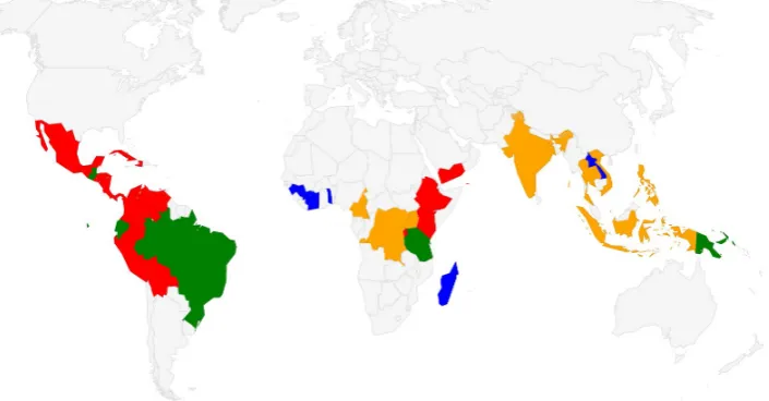
Figure 1: Coffee producing countries across the globe. Only countries with at least 0.05% of the total world production are shown. Data refer to 2014 production as provided by ICO web site (http://www.ico.org). Countries have been coloured as follows: Red for Arabicas milds, green for mixed products but mainly Arabicas, blue for Robustas and orange for mixed products but mainly Robustas.

As with many other primary commodities, the global coffee market has been defined by high volatility. Several sectors of the food industry are sensitive to prince transmission processes along the production, manufacturing and retail chains (Bakucs et al., 2014; Vavra and Goodwin, 2005) There is cumulative evidence that price transmissions can be asymmetric in many cases and that these asymmetries can be affected by several economic factors. Cointegration and meta-regression analysis have been routinely applied in the past to test for asymmetric price transmissions in a variety of commodities (Frey and Manera, 2007). There is strong evidence in the literature that several type of asymmetries exist and various econometric mod-els can capture special sub-cases of asymmetries under certain conditions (Bakucs et al., 2014; Frey and Manera, 2007; Meyer and Cramon-Taubadel, 2004; Rapso-manikis et al., 2006; Swinnen and Vandeplas, 2014).

demand. A recent research on this topic (Ubilava, 2012) has revealed that El Ni˜no Southern Oscillation (ENSO) influences coffee prices. Moreover there is strong ev-idence that price dynamics have non-linear characteristics and there is evev-idence of asymmetries at price transmissions at the farm/wholesale/retail levels (Mehtaa and Chavasb, 2008).

Despite coffee’s significant importance as a commodity, most of studies have been carried out considering aggregate commodity prices of the two coffee varieties, namely Arabicas and Robustas. The objective of this study is to empirically exam-ine the nature of price dependence between different qualities of coffee. To examexam-ine such possible dependencies we utilized the copula methodology (Joe, 2014; Nelsen, 2007), Copulas are a useful tool in order to investigate bivariate interdependen-cies of economic data (Joe, 2014; Meucci, 2011; Nelsen, 2007; Patton, 2012). More specifically, copulas are used to model the joint behavior of random variables during extreme market events, making it possible to assess whether prices move with the same intensity during market upswings and downswings. If prices boom and crash together, there is no evidence of asymmetric price dependence, and this is an indi-cator of a well functioning market. If prices in different markets do not boom but crash together (and vice versa), then there is evidence of asymmetry in the nature of price dependence. A significant advantage of copulas is that they allow the joint behavior of random processes to be modeled independently of the marginal distri-butions, providing this way considerable flexibility in empirical research (Joe, 2014; Patton, 2012).

in-terdependence is stronger that the more past years (Reboredo, 2012). Very recently copula based models have been applied in agricultural research to investigate price dependencies (Emmanouilides and Fousekis, 2015; Panagiotou and Stavrakoudis, 2015).

2

Methodology

Copula theory dates back to Sklar (1959), but only recently copula models have realized widespread application in empirical models of joint probability distributions (see Joe (2014); Nelsen (2007) for more details). The models use a copula function to tie together two marginal probability functions that may or may not be related to one another.

A two–dimensional copula, C(u1, u2), is a multivariate distribution function in

the unit hypercube [0,1]2 _{with uniform U(0,1) marginal distributions.}2 _{As long as}

the marginal distributions are continuous, a unique copula is associated with the joint distribution, H, and is described in equation (1). This function constitutes a form of the principal result of copula theory (Sklar’s theorem). It is obtained as:

C(u1, u2) = H(H1−1(u1), H2−1(u2)) (1)

Similarly, given a two-dimensional copula, C(u1, u2), and two univariate

distri-butions, H1(x) and H2(x), equation 1 is a two-variate distribution function with

marginals H1(x) and H2(x), whose corresponding density function can be written

as:

h(x, y) =c(H₁(x), H₂(y))h₁(x)h₂(y), (2)

where the functions h1 and h2 are the densities of the distribution functions H1

and H2 respectively.

The density function of the copula, c, given its existence, can be derived using equation 1 and marginal density functions,hi:

c(u₁, u₂) = h(H

−1

1 (u1), H2−1(u2)) h1(H1−1(u1))h2(H2−1(u2))

(3)

2

For simplicity we consider the bivariate case. The analysis, however, can be extended to a

A rank based test of functional dependence is Kendall’s τ. It provides informa-tion on co-movement across the entire joint distribuinforma-tion funcinforma-tion, both at the centre and at the tails of it. It is calculated from the number of concordant (PN) and

dis-concordant (Q_N) pairs of observations in the following way:

τ_N = PN −_NQN

2

=

4PN

N(N ₋1) −1, (4)

Often though, information concerning dependence at the tails (at the lowest and the highest ranks) is extremely useful for economists, managers and policy makers. Tail (extreme) co-movement is measured by the upper, λU, and the lower,

λL, dependence coefficients, such that λU, λL ∈[0,1], which are defined as

λU = lim

u↑1prob(U1 > u|U2 > u) = limu→1

1₋2u+C(u, u)

1₋u (5)

λL = lim

u↓0prob(U1 < u|U2 < u) = limu→0

C(u, u)

u (6)

where, given the random vector (X,Y) with marginal distribution,U₁for X (resp.

U₂ for Y),λ_U measures the probability that X is above a high quantile given thatY

is also above that high quantile, whileλL measures the probability thatX is below

a low quantile given thatY is also below that low quantile. In order to have upper or lower tail dependence, λU or λL need to be strictly positive. Otherwise, there

is upper or lower tail independence. Hence, the two measures of tail dependence provide information about the likelihood for the two random variables to boom and to crash together. For example, in our work, positive upper and zero lower tail dependence estimates would provide evidence that big increases in wholesale prices are matched at the retail level, whereas extreme negative shocks at the wholesale level are less likely to be transmitted to the retail level.

members of the elliptical copulas and Archimedean copulas, since they permit con-siderable flexibility in capturing price dependence between different cuts of beef be-tween wholesale and retail level in the US beef industry. Elliptical and Archimedean copulas are the two of the most commonly used copula families. The elliptical cop-ulas that we evaluate are the Gaussian (or Normal) and Student–t. Among the one parameter Archimedean copulas we consider there are the Clayton, Gumbel, Frank, and Joe. Clayton-Gumbel, Joe-Gumbel, Joe-Clayton and the Joe-Frank are among the two-parameter Archimedean copulas we examine.

Table 1 presents the copulas (Brechmann and Schepsmeier, 2013) under con-sideration in our study, their respective dependence parameters, their relationship to Kendall’s τ as well as to λ_U and λ_L (upper and lower dependence coefficients). From the elliptical copulas, the Gaussian copula is symmetric and exhibits zero tail dependence. Thus, irrespective of the degree of the overall dependence, extreme changes in one random variable are not associated with extreme changes in the other random variable. The t-copula exhibits symmetric non-zero tail dependence (joint booms and crashes have the same probability of occurrence). From the one parame-ter Archimedean copulas, the Clayton copula exhibits only left co-movement (lower tail dependence). The Gumbel and the Joe copulas exhibit only right co-movement (upper tail dependence). The Frank copula has zero tail dependence. From the two- parameter Archimedean copulas, the Gumbel-Clayton and the Joe-Clayton al-low for potentially asymmetric upper and al-lower co-movement. The Joe-Gumbel exhibits only right co-movement while the Joe-Frank exhibits zero tail dependence. Recently, dynamic or time-varying copula models have been applied in order to investigate time-varying dependence structure (Manner and Reznikova, 2012; Reznikova, 2012). In this study we tested for time-varying dependence using Kendall’s

Table 1: Copulas functions, parameters, kendall’s τ, tail dependence

Copulas Parameters Kendall’s τ Tail dependence (λL, λU)

Gaussian θ _∈(₋1,1) _π2arcsin(θ) (0,0)

Student - t θ _∈(₋1,1) _π2arcsin(θ) 2tν+1(−√ν+ 1

q

1−θ

1+θ),

v¿2 2tν+1(−√ν+ 1

q

1−θ

1+θ)

Clayton θ > 0 θ

θ+2 (2

−1

θ , 0)

Gumbel θ _≥1 1- 1_θ (0, 2 - 21θ)

Frank θ _∈R_\{0_} 1 -4

θ + 4 D(θ)

θ (0,0)

Joe θ _≥1 1+_θ42

R1

0 tlog(t)(1−t)

2(1−θ)/θ_{dt (0, 2 - 2}1

θ)

Clayton-Gumbel θ1 >0, θ2 ≥1 1 - _θ2(θ2₁₊₂₎ (2

−1 θ

1θ2, 2 - 2 1

θ

2)

Joe-Gumbel θ1 ≥1, θ2 ≥1 1+_θ14_θ2

R1

0(−log(1−(1−t)

θ1) (0, 2 - 2 1

θ

1θ2)

*(1₋t)(1₋(1₋t)−θ1))_dt

Joe-Clayton θ1 ≥1, θ2 >0 1+_θ4

1θ2

R1

0(−(1−(1−t)

θ1)θ2+1 (2− 1

θ

2, 2 - 2 1

θ

1)

*(1−(1−t)θ1)−θ₂₋₁

(1−t)θ

2−1 )dt

Joe-Frank θ_{1 ≥}1, θ_{2 ∈}(0,1] 1+_θ4

1θ2

R1

0(−log(

(1−tθ2)θ1−1

(1−θ2)θ1−1) (0, 0)

3

Data

Coffee prices were obtained from the International Coffee Organization website (ICO, 2015). The data are indicator prices (monthly averages expressed in USD cents per pound) of four different coffee qualities: ”Colombian Arabicas milds” (Colombian, or Col), ”Brazilian and other natural Arabicas” (Brazilian, or Bra), ”Other mild Arabicas” (Others, or Oth) and Robustas (Rob). The first three, namely Colombian, Brazilian and Others, are of the Arabica variety and considered to be of higher quality. Robustas is mainly produced by African countries and it is considered to be of relatively lower quality in comparison with the Arabicas.

The time period we consider in this study is from 1990:1 to 2014:12. Figure 2 presents the time evolution of coffee prices for the four coffee qualities considered in our study. As we can observe, prices appear to move together: price increases and price decreases follow similar patterns. Colombian coffee (red continued line of Figure 2) constitutes the upper bound, which is in consistency with the fact that it is considered to be of higher quality. In contrast, lower quality Robustas (blue dashed line of Figure 2) lies on the lower bound of the four time series. Brazilian and Other Milds are of intermediate quality thus their time series lie between Colombian and Robustas. It must be noted that the estimation period starts shortly after the collapse of the International Coffee Agreement (ICA), when the export quotas were eliminated, and prices have since been determined under the free market conditions. Monthly returns from coffee prices have been calculated as the percentage of value change according to the formula:

r_t= xt−xt−1

xt ×

100 (7)

wherext is the indicator coffee price. These return data have been used for further

estimation purposes.

Figure 2: Plot of coffee prices (USD cents per lb).

Table 2: Descriptive statistics of the coffee prices returns (values as percentages). P-values are displayed for the Kolmogorov-Smirnov (KS) and Cramer von Misses test for normality. Q(24) lists the p-values of the Ljung-Box test for time series independence taking into consideration 24 lags. ARCH-LM lists p-values of the autoregressive conditional heteroskedasticity–Lagrange multiplier test, also using 24 lags.

descriptive statistics. The Kolmogorov-Smirnov (KS) and Cramer von Misses tests reject normality. The p-values of the Ljung-Box test indicate that the data are not independently distributed.

Time

Retur

n (%)

−5 0 5

1990 1995 2000 2005 2010 2015

Robustas

Other

Colombian

1990 1995 2000 2005 2010 2015

−5 0 5

Brazilian

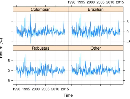
Figure 3: Plot of price returns.

Figure 4 shows the density distribution of the return data of the four coffee prices along the ideal normal distribution curve for comparison. It is evident from this graph that distribution of returns of the four coffee prices deviate from normality. This was also confirmed by examining the p-values of the Kolmogorov-Smirnov and Cram´er–von Mises normality tests depicted at Table 2.

0.00

0.10

0.20

0.30

return

density

−8 −4 0 4 8

Col Oth Bra Rob Normal

Figure 4: Density plot of price returns for the four coffee qualities. corre-sponding line of normal distribution (think magenta line) has been computed with mean=0.074 and sd=1.692, these values were obtained from mean and standard deviation of combined price returns of the four coffee time series.

Table 3: Correlation measurement between pairs of coffee prices.

4

Empirical models

A three step, semi-parametric approach has been applied for the empirical part of this article as proposed by Chen and Fan (2006):

1. An Autoregressive Moving Average – Generalized Autoregressive Conditional Heteroskedasticity (ARMA–GARCH) model is fit to the rates of price change for each of the series.

2. The standardized residuals are used to calculate the respective empirical dis-tribution functions, copula with range in (0,1).

3. The estimation of copula models is conducted by applying the maximum like-lihood (ML) estimator to the copula data (Canonical ML)

The semi-parametric approach exploits the fact that the copula and the margins can be estimated separately using potentially different methods. The Canonical ML copula estimator is consistent but less efficient relative to the fully parametric one. Hence, the asymptotic distributions of the copula parameters and the dependence measures, such as the Kendall’s τ and the tail coefficients, are approximated using resampling methods (Choro´s et al. (2010); Gaißer et al. (2010)). All estimations, testing, and resampling in this study have been carried out using R (version 3.1.2, R Core Team (2014)).

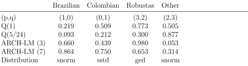
Table 4: Fitted ARMA(p,q)–GARCH(1,1) models of coffee price returns and test statistics of the residuals. First row (p,q) lists the ARMA order. Second row Q(1) lists the p-values of Lung–Box test with lag=1. Third row Q(5/24) lists the same but with lag=5 for models wherep+q= 1 and lag=24 wherep+q = 5. Rows ARCH(3) and ARCH(7) list p-values of the ARCH-LM test with 3 and 7 lags respectively. The last row lists the selected distribution of the residuals: snorm is the skewed normal distribution, sstd is the skewed student t distribution and ged is the generalized error distribution.

Brazilian Colombian Robustas Other (p,q) (1,0) (0,1) (3,2) (2,3) Q(1) 0.219 0.509 0.773 0.505 Q(5/24) 0.093 0.212 0.300 0.877 ARCH-LM (3) 0.660 0.439 0.980 0.053 ARCH-LM (7) 0.864 0.750 0.653 0.314 Distribution snorm sstd ged snorm

model for each of the series as well as the p-values produced from the application of the Ljung-Box (Q) and the autoregressive conditional heteroskedasticity–Lagrange multiplier (ARCH–LM) tests to the filtered data at various lag lengths. The ob-tained p-values reveal that the filtered data are free from autocorrelation and from ARCH effects.

The copula data was used in order to select the appropriate family function. Cop-ula family selection was performed with CDVine package (Brechmann and Schep-smeier, 2013) based on AIC/BIC criteria (Dißmann et al. (2013); Jordanger and Tjøstheim (2014); Manner (2007)). The same copula families were selected for all pairs in both criteria.

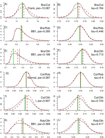
conver-gence.

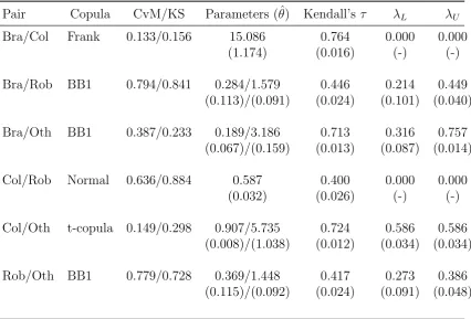
Table 5: Copula parameter estimates for the six pairs of different coffee qualities. CvM and KS are the p-values of the Cram´er–von Mises and Kolmogorov–Smirnov tests respectively. For Normal and Frank copulas one parameter is estimated (θ₁), for BB1 (Clayton–Gumbel) and t copulas two parameters (θ1, θ2) have been estimated.

Standard errors and standard deviations (in parentheses) were obtained with the bootstrap method.

Pair Copula CvM/KS Parameters (ˆθ) Kendall’s τ λ_L λ_U

Bra/Col Frank 0.133/0.156 15.086 0.764 0.000 0.000 (1.174) (0.016) (-) (-)

Bra/Rob BB1 0.794/0.841 0.284/1.579 0.446 0.214 0.449 (0.113)/(0.091) (0.024) (0.101) (0.040)

Bra/Oth BB1 0.387/0.233 0.189/3.186 0.713 0.316 0.757 (0.067)/(0.159) (0.013) (0.087) (0.014)

Col/Rob Normal 0.636/0.884 0.587 0.400 0.000 0.000 (0.032) (0.026) (-) (-)

Col/Oth t-copula 0.149/0.298 0.907/5.735 0.724 0.586 0.586 (0.008)/(1.038) (0.012) (0.034) (0.034)

Rob/Oth BB1 0.779/0.728 0.369/1.448 0.417 0.273 0.386 (0.115)/(0.092) (0.024) (0.091) (0.048)

5

Results and discussion

Table 5 presents the selected copula families for the six pairs of coffee milds. Kendall’s

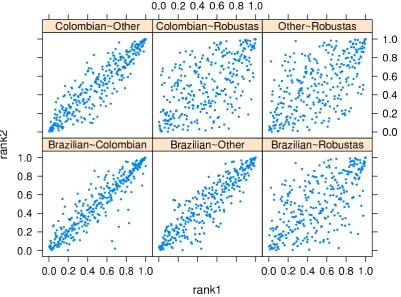
τestimates range from 0.400 to 0.764, and are statistically significant at the 1% level. The high values of kendall’s tau between the pairs Brazilian–Colombian (0.764), Brazilian–Others (0.713) and Colombian–Others (0.724) indicate the strong overall dependence between the three coffee qualities of the Arabica variety. This can also be seen in figure 5, where the scatterplots of the copula data (ranks) between the pairs formed between the three coffee qualities of the Arabica variety reveal their strong overall relationship. Overall dependence between the coffee qualities of the Arabica variety and the Robusta variety/quality is not as strong.

both tail dependence coefficients (λL,λU) are no different than zero. This means that

a price crash (boom) in one of the coffee qualities of the pair Brazilian–Colombian will not be associated with a price crash (boom) in the other coffee quality of the specific pair. The estimated value of Kendall’s τ is 0.764 and is the highest among the six pairs examined in this study, indicating this way the strongest overall de-pendence.

For the pair Brazilian–Robusta the Clayton-Gumbel (BB1) copula points to asymmetric tail dependence. The estimate of lower tail coefficient (λL) is 0.214, while

the estimated value of the upper tail coefficient (λU) is 0.449. The tail dependence

coefficients are statistically significant at any reasonable level. The value of λL

suggests that with a probability of 0.214 a strongly negative rate of price change in one of the two coffee qualities will be matched with a with a similarly strong negative rate of price change in the other coffee quality. On the other hand, the value ofλU indicates that with a probability of 0.449 Brazilian and Robusta prices

will boom together. The estimate of Kendall’sτ is 0.446.

The Clayton-Gumbel (BB1) copula was also selected for the pair Brazilian– Others. The value of the estimate for the lower tail dependence coefficient is 0.316 and the estimate for the upper tail dependence coefficient is 0.757. Both are statisti-cally significant at any reasonable level. The estimated values for the tail dependence coefficients suggest that with a probability of 0.214 the prices of the Brazilian and Other milds will crash together and with a probability of 0.449 a strongly positive rate of price change change in either one of the two coffee qualities of the Arabica variety will be matched with a with a similarly strong positive rate of price change in the other coffee quality. The estimate of the overall dependence parameter is 0.713.

be associated with a crash (boom) in the price of the Robusta, and vice versa. The estimate of Kendall’sτ is 0.400.

For the pair Colombian–Others, the student–t copula points to symmetric tail dependence, since λ_L and λ_U take the same value. The tail dependence coefficients suggest that coffee prices of Colombian and Other milds boom and crash together with a probability of 0.586. The estimate of Kendall’s τ is 0.724, indicating strong overall dependence.

For the pair Robusta–Others the Clayton-Gumbel (BB1) copula points to asym-metric tail dependence. The estimated value of lower tail dependence coefficient is 0.273, while the estimate of the upper tail dependence coefficient is 0.386. The tail dependence coefficients are statistically significant at any reasonable level. Their estimated values of λ_L and λ_U suggest that with a probability of 0.214 Brazilian and Robusta prices will crash together and with a probability of 0.449 the prices of Brazilian and Robusta will boom together. The estimate of Kendall’s τ is 0.446.

Our empirical findings reveal evidence of asymmetric price dependence between the pairs of Brazilian–Robusta, Brazilian–Others and Others–Robusta, since price booms and price crashes are transmitted with different probabilities between these three pairs of coffee qualities. On the other hand, for the pairs Brazilian–Colombian, Colombian–Robusta and Colombian–Others there is no evidence of asymmetric price dependence, since our results show that price booms (crashes) will be transmitted with the same probability. The probability price transmission is no different than zero for the pairs Brazilian–Colombian and Colombian–Robusta, and assumes the value of 0.586 for the pair Colombian–Others.

com-modities, coffee has been defined by high volatility and long-term declining prices. In order to alleviate the impacts of the low coffee prices sustainable coffee production and certification have been a logical choice for many producers. Coffee is generally regarded as the leading industry for sustainability standards and certification (Rei-necke et al., 2012). One of the pioneers in sustainability certification is Fairtrade. Fairtrade coffee production has to adhere to fairtrade standards. There are two types of generic standards: one for small producers and another for workers on plantations and in factories(Kilian et al., 2006). The first one applies to small-property own-ers organized into cooperatives or other types of organizations with a democratic and participatory structure. The second one applies to organized workers whose employers pay decent salaries, guarantee them the right to join unions and provide lodging when relevant. Fairtrade’s production has relied heavily on Latin Amer-ican sources, with an estimated 77 per cent of fairtrade coffee production coming from Latin American countries, where higher quality Arabica coffee is produced.3 _In

Colombia, Peru, and Nicaragua fairtrade represents 20 per cent or more of domestic production. At the same time, sales of fairtrade coffee are still experiencing growth, making it this way quite vulnerable to extreme events of price volatility.

Our empirical findings indicate that the price of the Colombian mild (highest Arabica quality) and Robusta price will neither crash nor boom together. This means that the probability that an extreme decrease in the prices of the Robusta quality will cause an extreme reduction in the prices of the Colombian quality of coffee is no different than zero. The Colombian quality belongs to the Arabica variety which is mainly produced in Latin America where the majority of faitrade coffee is produced.

On the other hand, the probability that a price crash in the price of the Robusta will cause a crash in the price of the Brazilian and the price of the Other milds of the Arabica variety is lower than the probability of the transmission of a price

3

boom between the pairs formed by these coffee qualities. This means that fairtrade coffee producers of these two qualities of the Arabica variety will see a price increase happening with much higher probability than a price decrease when extreme market conditions occur in the production of the Robusta coffee quality.

Figure 5: Scatterplots of the copula data (ranks). Data have been plotted as rank2_∼rank1, with rank1 on the horizontal axis and rank2 on the vertical axis respectively.

6

Copula stability

12 14 16 18 20 0.0 0.2 0.4 Bra/Col Frank, par=15.087 A)

0.72 0.74 0.76 0.78 0.80 0.82

0 10 20 30 Bra/Col tau=0.764 B)

0.0 0.2 0.4 0.6 0.8

0 1 2 3 4 5 Bra/Rob BB1, par=0.285 C)

0.35 0.40 0.45 0.50 0.55

0 5 10 15 Bra/Rob tau=0.446 D)

0.1 0.2 0.3 0.4 0.5 0.6

0 2 4 6 8 Bra/Oth BB1, par=0.189 E)

0.66 0.68 0.70 0.72 0.74 0.76

0 10 20 30 Bra/Oth tau=0.713 F)

0.45 0.50 0.55 0.60 0.65 0.70 0.75

0 4 8 12 Col/Rob Normal, par=0.587 G)

0.30 0.35 0.40 0.45 0.50

0 5 10 15 Col/Rob tau=0.4 H)

0.88 0.89 0.90 0.91 0.92 0.93 0.94

0

20

40 Col/Oth

t, par=0.907 I)

0.68 0.70 0.72 0.74 0.76 0.78

0 10 20 30 Col/Oth tau=0.724 J)

0.1 0.2 0.3 0.4 0.5 0.6 0.7 0.8

0 1 2 3 4 Rob/Oth BB1, par=0.369 K)

0.35 0.40 0.45 0.50

0 5 10 15 _Rob/Oth tau=0.417 L)

Lag

K

endall’s tau

0.4 0.5 0.6 0.7

0 10 20 30

Brazilian/Colombian Brazilian/Other

0 10 20 30

Colombian/Other Brazilian/Robustas

0 10 20 30

Colombian/Robustas

0.4 0.5 0.6 0.7

Robustas/Other

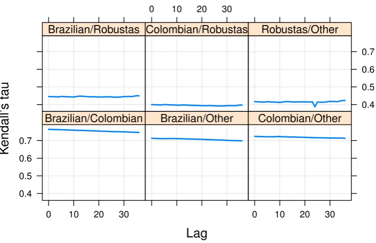
Figure 7: Plot of Kendall’sτ estimator with 36 lags

provides information on the co–movement at the center and at the tails of the joint distribution function. Hence, we test for time-varying dependence using Kendall’s

τ estimation over a rolling window (Zhang and Gu´eganc, 2008) of the price time series over 36 periods (month by month).

7

Conclusions

There is emerging consensus that the international agri-food system is becoming more vulnerable to extreme events of price volatility. Asymmetries in the transmis-sion of price volatility has always been in the center of attention in agricultural and food economics, since this might be an indicator of economic inefficiency.

In the coffee market, the abandonment of coffee quotas regulated by the Inter-national Coffee Agreement in 1989 led to a worldwide fall in producer prices for coffee. In the mid–nineties coffee prices recovered for some time but in the late 1990s coffee prices decreased drastically to their lowest real levels of the century (Kilian et al., 2006). Coffee as a world commodity, is second only to oil. Despite its importance as a commodity, most of studies have been carried out considering aggregate commodity prices of the two coffee varieties/species, namely Arabica and Robusta.

In this context, the objective of this work was to assess the nature of price depen-dence between four different coffee qualities: Colombian Arabicas milds, Brazilian and other natural Arabicas, Other mild Arabicas and Robustas. The first three are of the Arabica variety and considered to be of higher quality. Robusta is mainly produced by African countries and it is considered to be of relatively lower quality in comparison with the Arabica. The statistical methodology we used was that of copulas. Copulas are a useful tool in order to investigate bivariate interdependen-cies of economic data. Our results reveal evidence of asymmetric price dependence between the pairs Brazilian–Robusta, Brazilian–Others and Others–Robusta, since price booms and price crashes are transmitted with different probabilites between these three pairs of coffee qualities. On the other hand, for the pairs Brazilian– Colombian, Colombian–Robusta and Colombian–Others there is no evidence of asymmetric price dependence.

as the fairtrade scheme of coffee certification. Seventy–seven per cent of fairtrade coffee production comes from Latin American countries, where higher quality Ara-bica coffee is produced. According to the results of this work, the probability that fairtrade coffee producers will see a price crash in the Robusta variety being trans-mitted to the Arabica variety is either zero (Col/Rob) or much lower than the probability of the transmission of a price boom (Bra/Rob, Rob/Oth).

References

Acar, E. F., C. Genest, and J. NeˇsLehov´a (2012). Beyond simplified pair-copula constructions. Journal of Multivariate Analysis 110, 74–90.

Akiyama, T. and P. N. Varangis (1990). The impact of the international coffee agreement on producing countries. The World Bank Economic Review 4, 157– 173.

Bacon, C. M., V. E. Mendez, S. R. Gliessman, D. Goodman, and J. A. Fox (Eds.) (2008).Fair Trade, Sustainable Livelihoods and Ecosystems in Mexico and Central America . MIT Press.

Bakucs, Z., J. Fa lkowski, and I. Fert˝o (2014). Does Market Structure Influence Price Transmission in the Agro-food Sector? A Meta-analysis Perspective. Journal of Agricultural Economics 65, 1–25.

Berg, D. (2009). Copula goodness-of-fit testing: an overview and power comparison.

The European Journal of Finance 15, 675–701.

Brechmann, E. C. and U. Schepsmeier (2013). Modeling Dependence with C- and D-Vine Copulas: The R Package CDVine. Journal of Statistical Software 52, 1–27.

Byrd, R. H., P. Lu, J. Nocedal, and C. Zhu (1995). A limited memory algorithm for bound constrained optimization. SIAM Journal on Scientific Computing 16, 1190–1208.

Chen, X. and Y. Fan (2006). Estimation of copula-based semiparametric time series models. Journal of Econometrics 130, 307–335.

Czado, C., U. Schepsmeier, and A. Min (2012). Maximum likelihood estimation of mixed c-vines with application to exchange rates. Statistical Modelling 12(3), 229–255.

Dißmann, J., E. Brechmann, C. Czado, and D. Kurowicka (2013). Selecting and es-timating regular vine copulae and application to financial returns. Computational Statistics & Data Analysis 59, 52 – 69.

Donnet, M. L., D. D. Weatherspoon, and J. P. Hoehn (2008). Price determinants in top-quality e-auctioned specialty coffees. Agricultural Economics 38, 103–118.

Emmanouilides, C. J. and P. Fousekis (2015). Vertical price dependence structures: copula-based evidence from the beef supply chain in the USA. European Review of Agricultural Economics 42, 77–97.

Frey, G. and M. Manera (2007). Econometric models of asymmetric price transmis-sion. Journal of Economic Surveys 21, 349–415.

Gaißer, S., M. Ruppert, and F. Schmid (2010). A multivariate version of Hoeffding’s phi-square. Journal of Multivariate Analysis 101, 2571–2586.

Genest, C. and W. Huang (2012). A regularized goodness-of-fit test for copulas.

Journal de la Soci´et´e Fran¸caise de Statistique & revue de statistique appliqu´ee 154, 64–77.

Genest, C., B. R´emillard, and D. Beaudoin (2009). Goodness-of-fit tests for copulas: A review and a power study.Insurance: Mathematics and Economics 44, 199–213.

Ghalanos, A. (2014). rugarch: Univariate GARCH models. R package version 1.3-4.

Ghoshray, A. (2009). On Price Dynamics for Different Qualities of Coffee. Review of Market Integration 1, 103–108.

ICO (2015). International coffee organization. http://www.ico.org. Accessed 16 February 2015.

Joe, H. (2014). Dependence Modeling with Copulas. CRC Press.

Jordanger, L. A. and D. Tjøstheim (2014). Model selection of copulas: AIC versus a cross validation copula information criterion. Statistics & Probability Letters 92, 249–255.

Kilian, B., C. Jones, L. Pratt, and A. Villalobos (2006). Is sustainable agriculture a viable strategy to improve farm income in Central America? A case study on coffee. Journal of Business Research 59, 322–330.

Kojadinovic, I., J. Yan, M. Holmes, et al. (2011). Fast large-sample goodness-of-fit tests for copulas. Statistica Sinica 21, 841–871.

Manner, H. (2007). Estimation and model selection of copulas with an application to exchange rates. Technical report. http://arnop.unimaas.nl/show.cgi?fid=9426.

Manner, H. and O. Reznikova (2012). A Survey on Time-Varying Copulas: Specifi-cation, Simulations, and Application. Econometric Reviews 31, 654–687.

Mehtaa, A. and J.-P. Chavasb (2008). Responding to the coffee crisis: What can we learn from price dynamics? Journal of Development Economics 85, 282–311.

Meucci, A. (2011). A Short, Comprehensive, Practical Guide to Copulas. http://ssrn.com/abstract=1847864.

Meyer, J. and S. Cramon-Taubadel (2004). Asymmetric price transmission: a survey.

Journal of Agricultural Economics 55, 581–611.

Nash, J. C. and R. Varadhan (2011). Unifying Optimization Algorithms to Aid Software System Users: optimx for R. Journal of Statistical Software 43, 1–14.

Nelsen, R. B. (2007). An introduction to copulas. Springer.

Paige, J. M. (1997). COFFEE AND POWER. Harvard University Press.

Panagiotou, D. and A. Stavrakoudis (2015). Price asymmetry between different pork cuts in the USA: a copula approach. Agricultural and Food Economics 3(1).

Patton, A. J. (2012). A review of copula models for economic time series. Journal of Multivariate Analysis 110, 4–18.

Ponte, S. (2002). The ‘Latte Revolution’ ? Regulation, Markets and Consumption in the Global Coffee Chain. World Development 30, 1099–1122.

R Core Team (2014). R: A Language and Environment for Statistical Computing. Vienna, Austria: R Foundation for Statistical Computing.

Rapsomanikis, G., D. Hallam, and P. Conforti (2006). Market integration and price transmission in selected food and cash crop markets of developing countries: review and applications. In A. S. and D. Hallam (Eds.), Agricultural Commodity Markets and Trade, pp. 187–217. Edwar Elgar Publishing Limited.

Reboredo, J. C. (2011). How do crude oil prices co-move?: A copula approach.

Energy Economics 33, 948–955.

Reboredo, J. C. (2012). Do food and oil prices co-move? Energy Policy 49, 456–467.

Reinecke, J., S. Manning, and O. Von Hagen (2012). The emergence of a standards market: Multiplicity of sustainability standards in the global coffee industry. Or-ganization Studies 33(5-6), 791–814.

Reznikova, O. (2012). On the estimation of dynamic conditional correlation models.

Russell, B., S. Mohan, and A. Banerjee (2012). Coffee Market Liberalisation and the Implications for Producers in Brazil, Guatemala and India. The World Bank Economic Review 26, 514–538.

Sklar, A. (1959). Fonctions de r´epartition `A n dimensions et leurs marges. Publica-tons de L’Institut Statistique de L’Universite de Paris 8, 229–231.

Sukcharoen, K., T. Zohrabyan, D. Leatham, and X. Wu (2014). Interdependence of oil prices and stock market indices: A copula approach. Energy Economics 44, 331–339.

Swinnen, J. F. M. and A. Vandeplas (2014). Price Transmission and Market Power in Modern Agricultural Value Chains. http://dx.doi.org/10.2139/ssrn.2400431.

Talbot, J. M. (2004). Grounds for Agreement: The Political Economy of the Coffee Commodity Chain. ROWMAN & LITTLEFIELD PUBLISHERS.

Trivedi, P. K. and D. M. Zimmer (2005). Copula Modeling: An Introduction for Practitioners. Foundations and Trends in Econometrics 1, 1–111.

Ubilava, D. (2012). El Ni˜no, La Ni˜na, and world coffee price dynamics. Agricultural Economics 43, 17–26.

Vavra, P. and B. K. Goodwin (2005). Analysis of Price Transmission Along the Food Chain. http://dx.doi.org/10.1787/752335872456.

Wilson, A. P. and N. L. Wilson (2014). The economics of quality in the specialty cof-fee industry: insights from the Cup of Excellence auction programs. Agricultural Economics 45, 91–105.

Yan, J. (2007). Enjoy the Joy of Copulas: With a Package copula. Journal of Statistical Software 21, 1–21.