Short-term Traffic Forecasting Based on Grey
Neural Network with Particle Swarm Optimization
Yuanyuan Pan, Yongdong Shi
Abstract—An accurate and stable short-term traffic fore-casting model is very important for intelligent transportation systems (ITS). The forecasting results can be used to relieve traffic congestion and improve the mobility of transportation. This paper proposes a new hybrid model of grey system theory and neural networks with particle swarm optimization, namely, GNN-PSO. The proposed hybrid model can exploit sufficiently the characteristics of grey system model requiring less data, the non-linear map of neural networks and the quick-speed convergence of PSO, and has simpler structure. The GNN-PSO model is applied to predict the average speed of vehicle on Barbosa road in Macao. The experiment results show that the proposed model has better performance than grey forecasting model GM(1,1), back-propagation neural network model BPNN, and the combined model of them, i.e., grey neural network model (GNN), on short-term traffic forecasting.
Index Terms—Short-term traffic forecasting, Grey system, Neural networks, Grey neural network, Particle Swarm Opti-mization (PSO).
I. INTRODUCTION
S
HORT-TERM traffic forecasting is a vital component of intelligent transportation systems (ITS), which is a pro-cess of estimating directly the anticipated traffic conditions at a future time (usually time span less than 15 minutes) given continuous short-term feedback of traffic information. The most commonly used variables in traffic forecasting are three fundamental macroscopic traffic parameters: flow, occupancy and speed [1]. The forecasting results for these parameters can be used to assist traffic control center in ITS to reduce traffic congestion and improve the mobility of transportation [2]. Therefore, it is very significant for the development of ITS to predicate effectively and accurately short-term traffic information.In the last two decades, many scholars have devoted themselves to study this issue. Generally, the short-term traffic forecasting approaches can be divided into three cate-gories: statistical, artificial intelligence and hybrid methods. In the conventional statistical methods, Kalman filtering [3], autoregressive integrated moving average (ARIMA) [4] and seasonal ARIMA [5] have been applied to forecast short-term traffic flow based on past data. Although these statistical techniques can achieve reasonable prediction accuracy, they may not capture the dynamics and nonlinearities existed in traffic flow. To address this issue, the artificial intelligence methods, namely, neural networks (NNs) [6] [7] [8] [9], are widely used to the predication of short-term traffic flow due to its advantages of non-linear mapping relations
Manuscript received June 28, 2016; revised July 28, 2016. This work was supported by the Doctoral Scientific Research Foundation of Hubei University of Technology under Grant BSQD14036.
Y. Pan is with School of Computer Science, Hubei University of Tech-nology, Wuhan, 430070, China.
Y. Shi is with School of Business, Macau University of Science and Technology, Macao SAR, China. E-mail: [email protected].
[10]. However, NNs require a great deal of training data and relatively long training period for robust generalization [11] [12]. To enhance the generalization capability of NNs, several previous studies have proposed hybrid NNs models by incorporating genetic algorithms [13], fuzzy logical [14] [15], Kalman filters [16], the ARIMA model [17], and so on. These hybrid models have been demonstrated to possess better performance than pure NNs in short-time traffic fore-casting, but they use more parameters, have more complex structure and require greater computational power [18].
To address these issues, this paper proposes a new hybrid model of grey system theory and neural networks with par-ticle swarm optimization, namely, GNN-PSO. Grey system theory was first introduced in early 1980s by Deng. Since then, the theory has been widely used to forecast in various fields, such as agriculture, industry and environment, because it is simple and requires only a limited amount of data to esti-mate the behavior of uncertainty system. Neural networks, as above mentioned, has been a primary non-linear forecasting method because of its ability of self-learning, non-linear map and parallel distributed manipulation. Particle swarm optimization (PSO), as a global optimization technique, is used to solve the commonly existing problems in NNs, such as the slow speed of convergence and the local minimum [19], by estimating the parameters of NNs. As a result, the proposed hybrid model has the characteristics of grey system theory requiring less data, the strong non-linear map of neural networks and the quick-speed convergence of particle swarm optimization. Furthermore, the structure of GNN-PSO is relatively simpler since it only executes an accumulated generating operation (AGO) and an inversely accumulated generation operation (IAGO), which are derived from grey system theory, before and after neural network, respectively. To evaluate the performance of the GNN-PSO model, it is used to predict short-term traffic speed on Babosa road in Macao. Results show that the proposed hybrid model is more accurate and stable than the single grey model, the single neural network model and the combined model of them, i.e., grey neural network model (GNN).
This rest of this paper is organized as follows. Section II describes some fundamental concept about grey system theory, neural networks and PSO. Section III illustrates the mechanism of the GNN-PSO model. Section IV discusses the detailed experimental results. Section V finally concludes this paper.
II. FUNDAMENTAL CONCEPTS
A. Grey model
in positive data sequences [12]. Since all the data of traffic speed are positive, GM(1,1) model can be used to forecast the future values of short-term traffic speed. The process of GM(1,1) can be divided into three stages. In the first stage, to smooth the randomness, the primitive data obtained from the system to form the GM(1,1) is subjected to an operator, named Accumulating Generation Operator (AGO) [20]. The differential equation of GM(1,1) is then solved to obtain the n-step ahead predicted value of the system in the second stage. Finally, using the predicted value, the Inverse Accumulating Generation Operator (IAGO) is applied to find the predicted values of original data. More details are as follows.
Stage 1: Let the original sequence be denoted byX(0).
X(0) ={x(0)(1), x(0)(2), ..., x(0)(n)}, n≥4. (1)
On the basis of X(0), a new sequence X(1) is generated by AGO as
X(1)={x(1)(1), x(1)(2), ..., x(1)(n)} (2)
wherex(1)(k) =∑k i=1x
(0)(i), k= 1,2,3, ..., n.
Stage 2: First-order differential equation of GM(1,1) model is given as
dX(1)
dt +aX
(1)=u (3)
The solution of Eq. (3) can be obtained by using the least square method. That is
b
x(1)(k+ 1) = [x(0)(1)−u
a]e
−ak+u
a (4)
where
[a, u]T = (BTB)−1BTY (5)
and
B =
−1 2(x
(1)(1) +x(1)(2)) 1
−1 2(x
(1)(2) +x(1)(3)) 1 ..
. ...
−1 2(x
(1)(n−1) +x(1)(n)) 1
(6)
Y = [x(0)(2), x(0)(3), ..., x(0)(n)]T. (7)
Stage 3: IAGO is applied to obtain the predicted value of the original data at time k+ 1,xb(0)(k+ 1), since the grey forecasting model is formulated by using the data of AGO rather than original data.
b
x(0)(k+ 1) = [x(0)(1)−u
a](1−e
a)e−ak (8)
. . . .
. .
. . .
x1
x2
xn
y1
ym
Input Layer Hidden Layer Output Layer
bj
o jh w ji
w
o h
[image:2.595.307.557.55.221.2]b
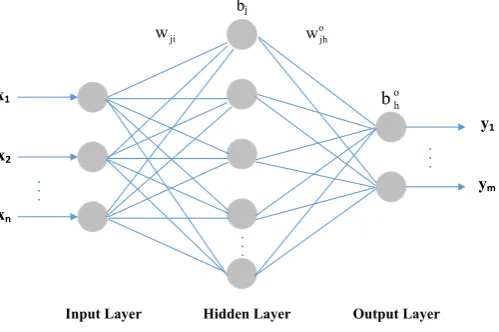
Fig. 1. The structure of BPNN
B. Neural networks
Back-propagation neural network (BPNN) is one of the most prevalent neural networks in short-term traffic fore-casting. It is based on a supervised learning algorithm which minimizes the global error by using the generalized delta rule and the gradient steepest descent method. The architecture of BPNN consists of an input layer, one or more hidden layers, and an output layer. Each layer comprises several neurons connected to the neurons in neighboring layers. Since BPNN contains many interacting nonlinear neurons in multiple layers, it can capture complex phenomena [21]. The parameters of BPNN include weights and biases which are adjusted iteratively by a process of minimizing the global error or the total square error. In this paper, BPNN is a three-layer network (one hidden three-layer) since the previous study [7], [8] have proved that the three-layer neural network can realize non-linear map for traffic flow. The structure of BPNN can be seen in Fig. 1, wherewji represents the connection weight from input node i to hidden nodej,wo
jh represents the connection weight from hidden nodejto output nodeh, bj stands for the bias of hidden nodejandbohstands for the bias of output nodeh.
C. Particle Swarm Optimization
As a population based stochastic optimization technique, Particle Swarm Optimization (PSO) was introduced by Kennedy and Eberhart in 1995. It is inspired by the social behavior of animals, such as bird flocking and fish schooling [22]. In PSO, each particle is a solution to an optimization problem. All the particles are initially distributed randomly over the search space, and then fly at certain velocity in the search space to find the global best position, namely, the global optimum, after some iterations. Suppose the dimen-sion of search space isDand the number of particles isN. The position and velocity of particleiat iterationtare denot-ed byXt
i ={xti1, xti2, ..., xtiD} andVit={vit1, vti2, ..., vtiD} (i = 1,2, ..., N), respectively. The best position of particle i and all particles at iteration t can be represented by Pbest,it ={Pit1, Pit2, ..., PiDt } andGtbest={Gt1, Gt2, ..., GtD}, respectively. The algorithm can be described as follow.
Step 2. Calculate the fitness value of each particlei. If its fitness value is better than the best fitness value in history, this value is set as the new best fitness value, and the current positions of this particle is set as its best positions Pbest.
Step 3. Compare all particles’ best fitness values and choose the particle with the best fitness value of them as the Gbest.
Step 4. Update the velocity and position of each particle i according to the next two equations.
Vit+1=ωVit+c1r1(Pbest,it −X t
i) +c2r2(GtBest−X t i) (9)
Xit+1=Xit+Vit+1 (10)
where ω is the inertia weight, c1 and c2 are the cognitive and social acceleration constants which are initially set to 2 [23],r1andr2are uniformly distributed random numbers in the range [0, 1]. In addition, the velocity of the particle is limited to the range [Vmin,Vmax].
Step 5. While maximum iterations or minimum error criteria is not attained, loop back to Step 2 again.
III. THE HYBRIDGNN-PSOMODEL
In this paper, the proposed hybrid GNN-PSO model for short-term traffic forecasting not only combines grey model with neural networks to form Grey Neural Network (GNN), but also optimizes the GNN model with particle swarm optimization algorithm.
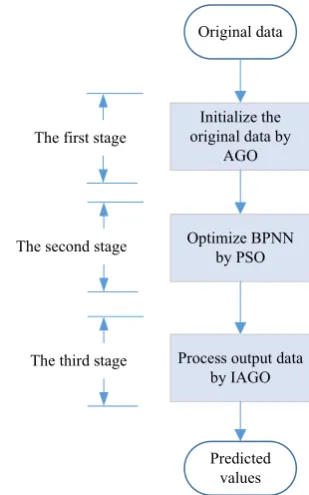
In the GNN-PSO model, there are three stages. The first stage initializes the original traffic speed series data by accumulating generation operator (AGO) in grey model in order to weaken the randomness of the original data, and then these data are feed into a back-propagation neural network (BPNN). The second stage focuses on the optimization of BPNN by using PSO algorithm to decide the optimal original value of parameters, such as weight and bias, in BPNN. In this stage, the structure of three-layer BPNN Nin ∗Nhindden ∗1 is first determined, where Nin refers to the number of data input from the first stage, 1 refers to the number of output forecasting value,Nhiddenrefers to the node number of hidden layer. According to the structure, the dimension of search space in PSO D is then decided, where D is equal to the number of all weights and biases in BPNN. In other words, for each particle, say particle i, its position can be expressed as Xi ={wmn, bm, whmo , b
o h} (1 ≤ n ≤ Nin, 1 ≤ m ≤ Nhidden, h = 1). The fitness function of particle i, denoted by f(Pi), is set to the error sum of squares between the predicted valuexb(0)(k+ 1)and the real value x(0)(k+ 1), which is expressed as follows.
f(Pi) =
1
M M
∑
k=1
(bx(0)(k+ 1)−x(0)(k+ 1))2 (11)
where M refers to the number of sample data. According to the steps of PSO algorithm as described above, the globe optimumGbest which is corresponding to the optimal weights and biases can be find. At last, BPNN that takes the
Original data
Initialize the original data by
AGO
Optimize BPNN by PSO
Process output data by IAGO
Predicted values The first stage
The second stage
[image:3.595.344.499.52.300.2]The third stage
Fig. 2. The structure of hybrid model GNN-PSO
weights and biases optimized by PSO as its initial parameters is trained continuously until the fixed iterations or the desired error is obtained. This aims to improve the robustness and accuracy of BPNN for short-term traffic forecasting. In the third stage, to obtain the predicted values, the output data from the optimized BPNN are processed by the inverse accumulating generation operator (IAGO) in grey model. The structure of hybrid model GNN-PSO is shown in Fig. 2.
IV. EXPERIMENT RESULTS
In this section, the proposed hybrid model GNN-PSO is used to forecast the future vehicular speed on Barbosa road in Macao during the period of PM 14:00-15:00, 19th August. The forecasting results are compared with that obtained from the single models, such as GM(1,1) and BPNN, and the combined model of them, i.e., Grey Neural Network (GNN) [24].
A. Data source
The speed data used for forecasting was collected by the real-time traffic information system which has been devel-oped by intelligent transportation systems (ITS) research laboratory of Macau University of Science and Technology. This system adopts dynamic data-collecting technology. The GPS terminals in 140 vehicles send data of the position and the speed of vehicles to the lab server in every 1 minute. The received data are saved in MySQL database. By calculating the arithmetic mean of the speed data in every last 3 minutes, we get the average real-time speed of vehicles in the road. So, we get 60 speed data totally that are calculated in every 1 minute between 14:00-15:00.
B. Data forecasting
TABLE I
THE COMPARISONS OF FORECASTING RESULTS
Time Actual data GNN-PSO GM BPNN GNN
Forecasting value
Relative error(%)
Forecasting value
Relative error(%)
Forecasting value
Relative error(%)
Forecasting value
Relative error(%) 14:51 21.245 20.644 2.83 19.049 10.34 18.474 13.04 20.089 5.44 14:52 29.275 22.916 21.72 21.789 25.57 24.376 16.74 25.445 13.08 14:53 30.92 29.708 3.92 29.248 5.41 33.057 6.91 23.334 24.53 14:54 27.95 27.73 0.79 28.209 0.93 38.172 36.57 22.973 17.81 14:55 21.75 24.229 11.40 22.035 1.31 32.752 50.58 27.062 24.42 14:56 14.34 15.468 7.87 18.908 31.86 21.957 53.12 12.243 14.62 14:57 10.88 11.886 9.25 14.394 32.30 13.123 20.61 16.075 47.75 14:58 15.80 8.311 47.40 12.244 22.51 7.9807 49.49 11.563 26.82 14:59 10.94 11.138 1.81 14.144 29.29 10.336 5.52 11.09 1.37 15:00 10.76 12.862 19.54 11.893 10.53 11.748 9.18 8.018 25.49
to 15:00 were divided into two sets. The first sub-set of the time series data, namely training data, collected from 14:00-14:50, were used for training the GNN-PSO model, the second sub-set of that, namely test data, collected from 14:51:15:00, were used to evaluate the generalization capability of this model. Whether training or evaluating, this model selects a time series data with equal dimension to predict the next data. The so-called equal dimension means, for a time series data, after predicting one traffic speed data, a new datum is added to the sequence at the end, meanwhile the oldest datum from the head of the sequence is take out, which results a new time series data with same dimension is generated to forecast the next traffic speed data. For example, using a time series data
{x(0)(k), x(0)(k+ 1), ..., x(0)(k+ 4)}, the GNN-PSO model predicts the value after one sampling times (i.e., 1 minutes) x(0)(k+ 5). In the next steps, the first data is always shifted to the second. It means that the model uses a time series data{x(0)(k+ 1), x(0)(k+ 2), ..., x(0)(k+ 5)}to forecast the value of x(0)(k+ 6). In this way, the new superseding the old, forecasting one by one, all need prediction results can be obtained. In this paper, the dimension of the time series data is set to 5. This means there are 45 and 10 pieces of speed data to train and validate the GNN-PSO model, respectively. In the GNN-PSO model, a time series data with 5 data are first selected to generate a new sequence by accumulated generating operation (AGO). The new sequence is used as the input data of BPNN. According to the number of input and output data, the structure of BPNN is decided as5∗Nhidden∗
1. Since the node number of hidden layer Nhidden is not the goal of this paper, we use one method recommended in [25], where Nhidden ≈log2(Ntr) with Ntr be the number of training data. As mentioned above,Ntr is equal to 45, so Nhidden is 6 in this case, i.e., log2(45)≈6. Based on the structure of BPNN, the dimension of search space in PSO is set to 43. The other parameters were used in PSO as follows: the population size of swarm is set to 20, the number of iterations is predefined as 200,ωis set to 0.8 and the training errors are below 10%. We use the optimum obtained by PSO as the initial parameters of BPNN, and then train again the optimized BPNN based on training data. The trained BPNN is used to forecast the last 10 data. Finally, we deal with the output 10 data of neural network by inverse accumulated generation operation (IAGO) to get the prediction value we need.
The performance of the hybrid GNN-PSO model is com-pared with the following models.
1) The single GM(1,1) model. Like the GNN-PSO model, the GM(1,1) model is built by using a time series data with 5 data and applying the equal dimension. But, due to no requirement of training neural network, the GM(1,1) model takes a time series data start from 14:46 to build grey model and forecast one data. This model iterates 10 times, then gives the last 10 speed forecasting results.
2) The single BPNN model. The structure and parameters of BPNN are identical to those of GNN-PSO. For instance, adopting 5 ∗ 6 ∗ 1 neural network, using Tansig as the transfer function between input layer and hidden layer, and applying Pureline for output layer. However, unlike GNN-PSO, the initial neurons connection weights of the single BPNN model are set to stochastic real number belonging to [-1, 1]. 3) The hybrid grey neural network (GNN) model. It has
three basic parts: a grey layer, a back-propagation neural network (BPNN), and a white layer [26]. The grey layer before neural network executes accumulated generating operation (AGO) to initialize input data. These new data generated by AGO are then feed into the neural network. Finally, the white layer after neural network inverses accumulated generation to the output data of the neural network. Therefore, the prediction value we need is obtained. The parameters used in GNN are identical to those used in GNN-PSO, except that there is no optimization in GNN by PSO.
The forecasting values and relative errors of the four models are as shown in Table I.
C. Evaluation and comparison
To investigating the viability of short-term traffic forecast-ing models, several performance measures have been applied in the previous studies. In this paper, the mean absolute percentage error (MAPE) and the root-mean-square error (RMSE) [18], shown as Eqs. (12) and (13), are used as the measures for comparison in these forecasting models. MAPE and RMSE respectively reflect the mean prediction accuracy and stability. The smaller MAPE is, the more accurate the prediction is. Similarly, the smaller RMSE is, the more stable the prediction is.
M AP E= 1
n n
∑
i=1
|xb(i)−x(i)
RM SE= 1
n v u u t∑n
i=1
(bx(i)−x(i)
x(i) )
2 (13)
wherex(i) is the actual value at theith time interval, bx(i)
is the forecasted value at the ith time interval, and nis the total number of the forecasted value.
Table II summarizes the results of MAPE and RMSE values obtained by the four models, i.e., GNN-PSO, GNN, GM(1,1) and BPNN. It can be seen that the MAPE value of GNN-PSO (12.65%) is the lowest, and decreases 25.6%, 51.67%, 37.17% compared to that of GNN, GM(1,1) and BPNN, respectively. This implies that the GNN-PSO model can improve the accuracy of forecasting short-term traffic speed. Furthermore, as shown in Table II, the RMSE values of GNN-PSO, GNN, GM(1,1) and BPNN are 3.33, 3.48, 6.22, 4.28, respectively. This indicates that GNN-PSO is more stable than other three model in short-term traffic forecasting. In a word, the results of MAPE and RMSE show that the proposed hybrid GNN-PSO model has the higher prediction accuracy and stability among the four models.
TABLE II
THEMAPEANDRMSEVALUES OF DIFFERENT MODELS
Criteria GNN-PSO GNN GM BPNN MAPE (%) 12.65 17.00 26.18 20.13 RMSE 3.33 3.48 6.22 4.28
V. CONCLUSION
In this paper, a new hybrid model of grey system theory and neural networks with particle swarm optimization, name-ly, GNN-PSO, has been proposed to predict short-term traffic speed. It aims to address some issues existed in the previous studies, including: (i) a great deal of history data; (ii) the non-linear characteristic of traffic data; (iii) the slow speed of convergence; (iv) great parameters and complex structure. The proposed model can be divided into three stages. In the first stage, the original traffic data are initialized by AGO in grey model to generate a new data sequence which is input into a BPNN. In the second stage, the BPNN is optimized by PSO algorithm. In the third stage, the data output from the optimized BPNN are processed by IAGO in grey model, thus the predicted values are obtained. This paper uses MAPE and RMSE to measure the accuracy and stability of forecasting models. The experimental results reveal that the predicted values obtained from GNN-PSO are more accurate and stable than that from the single GM(1,1), the single BPNN, and the combined model of them GNN. Of course, like most studies, the structure of GNN-PSO, such as the dimension of the time series data input into BPNN and the number of hidden nodes, is required to be pre-defined and fixed, which can not guarantee the optimal one will be obtained. How to optimize the structure of GNN-PSO with respect to time is left for our future work.
REFERENCES
[1] E. I. Vlahogianni, J. C. Golias, and M. G. Karlaftis, “Short-term traffic forecasting: Overview of objectives and methods,”Transport Reviews, vol. 24, no. 5, pp. 533–557, Sep. 2004.
[2] Y. Wang, M. Papageorgiou, and A. Messmer, “A real-time freeway network traffic surveillance tool,” IEEE Transactions on Control Systems Technology, vol. 14, no. 1, pp. 18–32, Jan. 2006.
[3] I. Okutani and Y. J. Stephanedes, “Dynamic prediction of traffic volume through kalman filtering theory,”Transportation Research Part B: Methodological, vol. 18, no. 1, pp. 1–11, Feb. 1984.
[4] B. L. Smith, B. M. Williams, and R. K. Oswald, “Comparison of parametric and nonparametric models for traffic flow forecasting,” Transportation Research Part C: Emerging Technologies, vol. 10, no. 4, pp. 303–321, Aug. 2002.
[5] B. M. Williams, P. K. Durvasula, and D. E. Brown, “Urban freeway traffic flow prediction: Application of seasonal autoregressive integrat-ed moving average and exponential smoothing models,” Transporta-tion Research Record: Journal of the TransportaTransporta-tion Research Board, 1998.
[6] M. Dougherty, “A review of neural networks applied to transport,” Transportation Research Part C: Emerging Technologies, vol. 3, no. 4, pp. 247–260, Aug. 1995.
[7] S. C. Chang, R. S. Kim, S. J. Kim, and M. H. Ahn, “Traffic flow forecasting using a 3-stage model,” inProc. of the IEEE Intelligent Vehicles Symposium 2000, Dearborn, USA, Oct. 2000, pp. 451–456. [8] H. Dia, “An object-oriented neural network approach to short-term
traffic forecasting,”European Journal of Operational Research, vol. 131, no. 2, pp. 253–261, Jun. 2001.
[9] C. Ledoux, “An urban traffic flow model integrating neural network,” Transportation Research Part C: Emerging Technologies, vol. 5, no. 5, pp. 287–300, Oct. 1997.
[10] S. Mao and X. Xiao, “Short-term traffic flow grey forecasting model gm(1,1 vertical bar tan(k-tau)p, sin(k-tau)p) of single-cross-section and its particle swarm optimization,”JOURNAL OF GREY SYSTEM, vol. 22, no. 4, pp. 383–394, 2010.
[11] T. C. Jo, “The effect of virtual term generation on the neural based approaches to time series prediction,” in Proc. 4th International Conference on Control and Automation (ICCA ’03), Montreal, Que., Canada, Jun. 2003, pp. 516–520.
[12] E. Kayacan, B. Ulutas, and O. Kaynak, “Grey system theory-based models in time series prediction,”Expert Systems with Applications, vol. 37, no. 2, pp. 1784–1789, Mar. 2010.
[13] E. I. Vlahogianni, M. G. Karlaftis, and J. C. Golias, “Optimized and meta-optimized neural networks for short-term traffic flow prediction: a genetic approach,”Transportation Research Part C: Emerging Tech-nologies, vol. 13, no. 3, pp. 211–234, Jun. 2005.
[14] H. Yin, S. C. Wong, J. Xu, and C. K. Wong, “Urban traffic flow prediction using a fuzzy-neural approach,”Transportation Research Part C: Emerging Technologies, vol. 10, no. 2, pp. 85–98, Apr. 2002. [15] C. Quek, M. Pasquier, and B. B. S. Lim, “Pop-traffic: A novel fuzzy neural approach to road traffic analysis and prediction,”IEEE Transactions on Intelligent Transportation Systems, vol. 7, no. 2, p. 133C146, Jun. 2006.
[16] D. Srinivasan, C. W. Chan, and P. G. Balaji, “Computational intelli-gence based congestion prediction for a dynamic urban street network,” Neurocomputing, vol. 72, no. 10, pp. 2710–2716, 2009.
[17] M.-C. Tan, S. C. Wong, J.-M. Xu, Z.-R. Guan, and P. Zhang, “An aggregation approach to short term traffic flow prediction,” IEEE Transactions on Intelligent Transportation Systems, vol. 10, no. 1, p. 60C69, Feb. 2009.
[18] K. Y. Chan, T. Dillon, E. Chang, and J. Singh, “Prediction of short-term traffic variables using intelligent swarm-based neural networks,” IEEE Transactions on Control Systems Technology, vol. 21, no. 1, pp. 263–274, Jan. 2013.
[19] J. ming Ma, Z. ren Xu, and B. zheng Wang, “A pso-based combined forecasting grey neural network model,” computer engineering & science, vol. 34, no. 2, pp. 146–149, 2012.
[20] J. L. Deng, “Introduction to grey system theory,”The Journal of Grey System, vol. 1, 1989.
[21] Y. Wei and M.-C. Chen, “Forecasting the short-term metro passen-ger flow with empirical mode decomposition and neural networks,” Transportation Research Part C, vol. 21, 2012.
[22] J. Hu and X. Zeng, “A hybrid pso-bp algorithm and its application,” inProc. 2010 Sixth International Conference on Natural Computation (ICNC 2010), vol. 5, Yantai, Shandong, China, Aug. 2010, pp. 2520– 2523.
[23] S. Kiranyaza, T. Inceb, A. Yildirimc, and M. Gabbouj, “Evolutionary artificial neural networks by multi-dimensional particle swarm opti-mization,” Neural Networks, vol. 22, no. 10, pp. 1448–1462, Dec. 2009.
[24] Y. dong Shi, Y.-Y. Pan, and J. qing Li, “Urban short-term traffic forecasting based on grey neural network combined model: Macao experience,” in Proc. 2009 International Workshop on Intelligent Systems and Applications (ISA 2009), Wuhan, China, May 2009, pp. 1–4.