Abstract—In this paper, we propose a handy approximation
technique (HAT) for obtaining both closed-form and approximate solutions of time-fractional heat and heat-like equations with variable coefficients. The method is relatively recent, proposed via the modification of the classical Differential Transformation Method (DTM). It devises a simple scheme for solving the illustrative examples, and some similar PDEs. Besides being handy, the results obtained converge faster to their exact forms. This shows that this modified DTM (MDTM) is very efficient and reliable. It involves less computational work, even without given up accuracy. Therefore, we strongly recommend it for solving both linear and nonlinear time-fractional partial differential equations (PDEs) with applications in other aspects of pure and applied sciences, management, and finance.
Index Terms— time-fractional differential equations;
modified DTM; heat and heat-like equations; variable coefficients, closed-form solutions.
I. INTRODUCTION
ANY physical problems in various fields of pure and applied sciences are modelled mathematically by partial differential equations. Heat equations are special version of parabolic partial differential equations (PPDEs) governing heat diffusion and heat-like diffusive processes.
Heat equations are of great importance in diverse areas of sciences and engineering. It is highly linked to the study of Brownian motion through the application of the Fokker-Planck equation (application in probability theory) [1]. In financial mathematics, the heat equation can also be used for the solutions of financial models like the Black-Scholes option pricing model [2], integro-differential model [3] and so on.
In the sequel, the heat equation will be generalized to the time-fractional case (that is, of non-integer order). The
Manuscript received January 29, 2016.
S.O. Edeki is with the Department of Mathematics, Covenant University, Canaanland, Otta, Nigeria: [email protected] (email of the corresponding author)
G.O. Akinlabii is with the Department of Mathematics, Covenant University, Canaanland, Otta, Nigeria.
A.O. Akeju is with the Department of Mathematics, University of Ibadan, Nigeria.
study of fractional calculus has greatly attracted the attention of many researchers because of its suitability for the generalization of fractional differential equations [4].
Fractional differential equations are seen as alternatives to non-linear differential equations [4]. Many researchers have proposed, adopted and applied various methods in search for solutions of heat and heat-like equations, and related PDEs [5-14]. Recently, while Secer [15] applied DTM to heat-like equations, we hereby propose the modified DTM for less computational work among other merits.
In this work, a relatively new version of the modification referred to as modified differential transform method (MDTM) will be applied to heat and heat-like PDEs for exact and numerical solutions. It is noteworthy saying that the MDTM has advantages over the decomposition methods and the classical DTM as the computational time required is minimal, and for ease and simplicity of usage.
II. FRACTIONAL CALCULUS:PRELIMINARIES AND
NOTATIONS
In fractional calculus, the power of the differential operator is considered a real or complex number. Hence, the following definitions [16-18]:
Definition 1: Fractional derivative in gamma sense
Let
D
d
and
J
dx
be differential and integral operators respectively, with the gamma function ofh x
( )
being defined as:1
0
( )
x n, Re( ) 0
n
e t
dt
n
,(
n
1)
n
!, (1/ 2)
(1) Equation (1) in terms of gamma sense is expressed as:
1
( )
( )
=
1
kk
d h x
D h x
x
dx
k
(2)Equation (2) is referred to as a fractional derivative of
( )
h x
, of order
, if
.Definition 2: Suppose
h x
( )
is defined forx
0
, then:A Handy Approximation Technique for
Closed-form and Approximate Solutions of
Time-Fractional Heat and Heat-Like Equations with
Variable Coefficients
S. O. Edeki, Member, IAENG, G. O. Akinlabi, and A.O. Akeju
0
( )
xJh
x
h s ds
(3) and as such, an arbitrary extension of (3) (i.e. Cauchy formula for repeated integration) yields:
1 01 !
(
)
( )
x
n n
n
J h
x
x
s
h s ds
(4) While the gamma sense of (4) is:
10
( ) ( ) , 0, 0.
x
J h x x s h s ds t
(5)Equation (5) is the Riemann-Liouville fractional integration of order
.Definition 3: Riemann-Liouville fractional derivative
( )
( )
d
J
h x
D h x
dx
(6)Definition 4: Caputo fractional derivative
( )
( ) J d f x , 1 ,
D f x
dx
(7)
In (6), Riemann-Liouville compute first, the fractional integral of the function and thereafter, an ordinary derivative of the obtained result but the reverse is the case in Caputo sense of fractional derivatives; this allows the inclusion of the traditional initial and boundary conditions in the formulation of the problem. The link between the Riemann-Liouville operator and the Caputo fractional differential operator [17, 19] is:
10
( ) ( ) ( ) (0)
!
k n
k
t t t
k
t J D h t D D h t h t h
k
(8)1
,
n
n n
As such,
10
( )
( )
(0)
!
k nk t
k
t
h t
J D
h t
h
k
(9)Definition 5: The Mittag-Leffler Function
The Mittag-Leffler function,
E
z
valid in the whole complex plane is defined and denoted by the series representation as:
0
,
0,
1
k
k
z
E
z
z
k
, (10)
1
z
E
z
e
for
1,
III. THE OVERVIEW OF THE MODIFIED DIFFERENTIAL TRANSFORM METHOD (MDTM)
The differential transformation method (DTM) has been studied by many researchers and showed to be easier in terms of application when solving both linear and nonlinear differential equations as it converts the said problems to their equivalents in algebraic recursive forms [6, 7, 9, 11, 15, 20]. This is unlike other semi-analytical methods: ADM, VIM, HAM and so on that require the determination of a successive term only by integrating a previous component.
In spite of the copious merits of the DTM over other semi-analytical methods, some levels of difficulties are still encountered when dealing mainly with nonlinearity of differential equations. This again creates rooms for modification of the DTM in various forms by many authors and researchers [21,22].
Let
x t, be an analytic function at
x t*,*
in adomain
D
, then in considering the Taylor series expansion of
x t, , regard is given to some variabless
ov
t
instead of all the variables as in the classical DTM. Thus, the MDTM of
x t, with respect to t at t* is defined anddenoted by:
* , 1
, !
h
h t t
x t x h
h t
(11)
And as such:
*
0
, , h
h
x h x h t t
(12) Equation (12) is called the modified differential inverse transform of
x h, with respect to t .A. Basic Theorems and properties of the MDTM [21].
Theorem a: If
x t, a
x t, b
x t, , then
x h, a
x h, b
x h,
Theorem b: If
, *
, tn
n
x x t
t
, then
*
!
, ,
!
h n
x h x h n
h
Theorem c: If
,
*
, tn
n
p x x
x t
x
, then
,
*
,n
n
p x x h
x h
x
Theorem d: (MDTM of a fractional derivative)
If
g x t
,
D
t
x t
,
, then
1
k
G x k
,
1
k
x k
,
q
q
q
,and:
1
k
x k
,
q
1
k
G x k
,
q
q
(13)Setting
q
1
in (13) yields (14) and (15) as follows:
,
1
1
,
1
1
k
x k
G x k
k
(14)As such, for
x t
, , -analytic at
x
0
0
0
,
,
hh
x t
x h t
(15)Consider the nonlinear fractional differential equation (NLFDE):
, , , , 0
,0 , 0
t x x
D x t L x t N x t q x t
w x g x t
(16)
where
D
tt
is the fractional Caputo derivative of
x t
,
; whose modified differential transform is( , )
x h
,L
and
N
are linear and nonlinear differential operators with respect tox
respectively, whileq
q x t
.
is the source term. We rewrite (16) as:
,
,
, , ,1 ,
t x x
D x t L x t N x t q x t
n n n
(17)
Applying the inverse fractional Caputo derivative,
D
t to both sides of (23) and with regard to (8) gives:
, ( ) ,
, , , ,0 ( )
t x
x
x t g x D L x t
N x t q x t x g x
(18)
Thus, expanding the analytical and continuous function,
( , )
x t
in terms of fractional power series, the inverse modified differential transform of
( , )
x h
is given as follows:
0 1, , ,0 , ,
,0 ( )
h h
h h
x t x h t x x h t
x g x
(19)
IV. ILLUSTRATIVE EXAMPLES AND APPLICATIONS
In this subsection, we will consider via the proposed method, the following initial boundary value problems (IBVPs) describing heat and heat-like PDEs of time-fractional orders.
A. Problem 4.1: Consider the time-fractional heat and heat-like equation {[6, 10, 13] for 1}:
22mt x mxx x t, , x
0,1 , t
0,
(20) subject to the boundary conditions (20a) and the initial condition (20b) below:
0, 0,
1, tm t m t e (20a)
,0 2m x x (20b)
Solution to problem 4.1:
We take the modified differential transform (MDT) of (20) and (20b) as follows:
2
2 t xx
MDT m x m & MDT m x
,0 x2 (21)
, 1 2 , ,0 22 1 1
0
1 x k x k x
k
M x M , k & M x
k
(22)
Thus,
2
, 1 ,
1
2 1 1
x k x k
k x M M k
, (23)
When
k
0
,
2 ,1 ,0 1 2 1 x x x M M
, Mx ,0 2
2 ,1 1 x x M
, & ,1
2 1 x M
(24)
When
k
1
,
2
,2 ,1
1 2 1 2
x x
x
M
M
2 ,2 1 2 x x M
& ,2
2 1 2 x M
(25)
When
k
2
,
2
,3 ,2
1 2 2 1 3
x x
x
M
M
2,3 1 3
x
x M
, & ,3
2 1 3 x M
(26)
It follows thus, for kn, we have:
2 , 1 1 1 x n x M n , & , 1
2 1 1 x n M n
(27) For n 1 (27) becomes:
2
, 1
x
x
M , & ,
2 1 x
M (28)
, ,
0 h
x t x h
h
m M t
Mx,0M tx,1 Mx,2t2 M tx,3 3
2 2 2 2 3
2
1 1 2 1 3
x t x t x t
x
2 4 2
1 4 1
x t x t
2 1 1 1 t x
2 0 1 t x
(29)Thus, by using definition 5, (29) becomes:
2
, x t
m x E t (30)
Remark: when
1
, the exact solution is therefore:2 ,
t x t
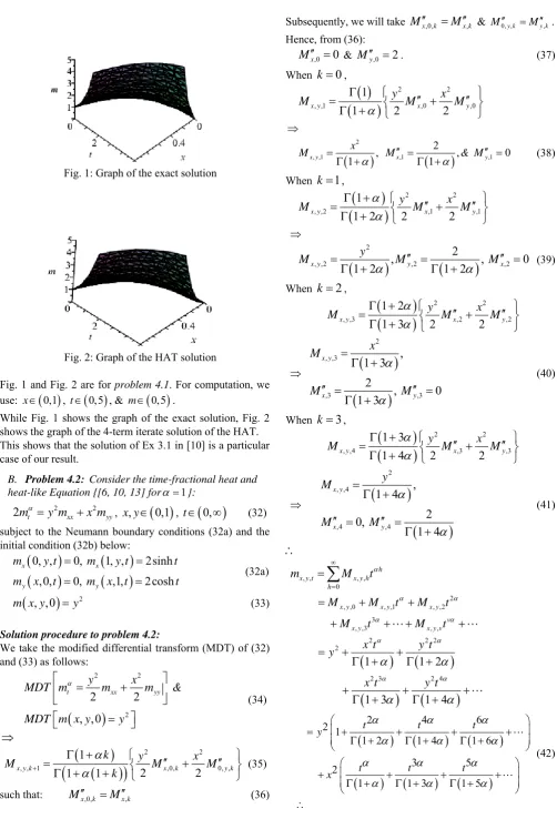
Fig. 1: Graph of the exact solution
Fig. 2: Graph of the HAT solution
Fig. 1 and Fig. 2 are for problem 4.1. For computation, we
use: x
0,1 , t
0,5 , & m
0,5 .While Fig. 1 shows the graph of the exact solution, Fig. 2 shows the graph of the 4-term iterate solution of the HAT. This shows that the solution of Ex 3.1 in [10] is a particular case of our result.
B. Problem 4.2: Consider the time-fractional heat and heat-likeEquation {[6, 10, 13] for 1}:
2 2
2mt y mxxx myy, x y,
0,1 , t
0,
(32) subject to the Neumann boundary conditions (32a) and the initial condition (32b) below:
0, , 0, 1, , 2sinh
,0, 0, ,1, 2cosh
x x
y y
m y t m y t t
m x t m x t t
(32a)
, ,0
2m x y y (33)
Solution procedure to problem 4.2:
We take the modified differential transform (MDT) of (32) and (33) as follows:
2 2
2
2 2
, ,0
t xx yy
y x
MDT m m m &
MDT m x y y
(34)
2 2
, , 1 ,0, 0, ,
1
2 2
1 1
x y k x k y k
k y x
M M M
k
(35)
such that: Mx,0,k Mx k, (36)
Subsequently, we will take Mx,0,k Mx k, & M0, ,y k My k, . Hence, from (36):
,0 0 x
M & My ,0 2. (37) When
k
0
,
2 2
, ,1 ,0 ,0
1
1 2 2
x y x y
y x
M M M
2
, ,1 ,1 ,1
2
, , 0
1 1
x y x y
x
M M & M
(38)
When
k
1
,
2 2
, ,2 ,1 ,1
1
1 2 2 2
x y x y
y x
M
M M
2
, ,2 ,2 ,2
2
, , 0
1 2 1 2
x y y x
y
M M M
(39)
When
k
2
,
2 2
, ,3 ,2 ,2
1 2
1 3 2 2
x y x y
y x
M
M M
2 , ,3
,3 ,3
, 1 3
2 , 0
1 3
x y
x y
x M
M M
(40)
When
k
3
,
2 2
, ,4 ,3 ,3
1 3
1 4 2 2
x y x y
y x
M
M M
2 , ,4
,4 ,4
, 1 4
2 0,
1 4
x y
x y
y M
M M
(41)
, , , ,
0
h
x y t x y h
h
m M t
2
, ,0 , ,1 , ,2
3
, ,3 , ,
x y x y x y
v
x y x y v
M M t M t
M t M t
2 2 2
2
2 3 2 4
1 1 2
1 3 1 4
x t y t y
x t y t
2 4 6
2 1
1 2 1 4 1 6
3 5
2
1 1 3 1 5
t t t
y
t t t
x
(42)
2 1 2
2 2
, ,
0 1 2 0 1 2 1
x y t
t t
m y x
(43)Remark: when
1
, (43) yields the exact solution to problem 4.2 as:2 2
, , sinh cosh
x y t
m x ty t (44) This is in agreement with {[6, 10, 13] for 1}.
V. CONCLUDING REMARKS
In this paper, we implemented a handy approximation technique as a modified DTM (MDTM) for the solutions of time-fractional heat and heat-like equations. For the efficiency and reliability of the proposed technique, some illustrative examples were used; both closed-form and approximate solutions were obtained. The solutions were very much in agreement. A simple recursive equation was obtained via the proposed technique. We therefore, conclude that MDTM boosts the effectiveness of the computational work when compared with the classical DTM, even without given up accuracy. Consequently, we recommend the technique for solving linear and nonlinear time-space-fractional PDEs with applications in other areas of pure and applied sciences, finance and management.
ACKNOWLEDGEMENT
With sincerity, the authors wish to thank Covenant University for financial support and provision of good working environment. The authors also wish to thank the anonymous referee(s)/reviewer(s) for their constructive and helpful remarks.
AUTHOR CONTRIBUTIONS
The concerned authors: SOE, GOA and AOA contributed positively to this work. They all read and approved the final manuscript for publication.
REFERENCES
[1] S.A. Adeosun and S.O. Edeki, “On a Survey of Uniform Integrability of Sequences of Random Variables”, International Journal of Mathematics and Statistics Studies,2 (1), (2014): 1-13.
[2] S.O. Edeki, O.O. Ugbebor, E.A. Owoloko, “Analytical Solutions of the Black–Scholes Pricing Model for European Option Valuation via a Projected Differential Transformation Method” Entropy, 17 (11), (2015): 7510-7521.
[3] S.O. Edeki, I. Adinya and O.O. Ugbebor, “The Effect of Stochastic Capital Reserve on Actuarial Risk Analysis via an Integro-differential Equation” IAENG International Journal of Applied Mathematics, 44 (2), (2014): 83-90.
[4] I. Podlubny, “Fractional Differential Equations”, Academic Press, (1999).
[5] A.M. Wazwaz, A. Gorguis, “Exact solutions of heat-like and wave-like equations with variable coefficients”, Appl. Math. Comput.149
(1), (2004): 15-29.
[6] Y. Keskin and G. Oturanc, “Reduced differential transform method for solving linear and nonlinear wave equations”, Iranian Journal of Science & Technology, Transaction A, 34, (A2), (2010).
[7] K. Tabatabaei, E. Celik and R. Tabatabaei, “The differential transform method for solving heat-like and wave-like equations with variable coefficients”, Turk. J. Phys. 36 (2012): 87-98.
[8] U. Filobello-Nino et al., “A handy approximate solution for a
squeezing flow between two infinite plates by using of Laplace
transform-homotopy perturbation method”, Springerplus, (2014) 3:
421.
[9] Z. Odibat, S. Momani, A generalized differential transform method for linear partial differential equations of fractional order, Applied Mathematics Letters, 21 (2008) 194–199.
[10] B. A. Taha, “The Use of Reduced Differential Transform Method for Solving Partial Differential Equations with Variable Coefficients”,
Journal of Basrah Researches (Sciences), 37, (4), C (2011). [11] S. Momani, “Analytical approximate solution for fractional heat-like
and wave-like equations with variable coefficients using the decomposition method”, Appl. Math. Comput. 165 (2), (2005):
459-472.
[12] S.T. Mohyud-Din, "Solving heat and wave-like equations using He's polynomials," Mathematical Problems in Engineering, (2009), Article ID 427516, (2009): 1-12.
[13] Y. Keskin, S. Servi and G. Oturanç, “Reduced Differential Transform Method for Solving Klein Gordon Equations”, Proceedings of the World Congress on Engineering (WCE), 2011, l (2011): July 6 - 8, London, U.K.
[14] H. Xu, J. Cang, “Analysis of a time fractional wave-like equation with the homotopy analysis method”, Phys. Lett. A, 372, (2008):
1250-1255.
[15] A. Secer, “Approximate analytic solution of fractional heat-like and wave-like equations with variable coefficients using the differential transforms method”, Advances in Difference Equations, 2012, (2012):198.
[16] M. Dalir, “Applications of Fractional Calculus”, Applied Mathematical Sciences, 4, (21), (2010): 1021-1032.
[17] F. Mainardi, “On the Initial Value Problem for the Fractional Diffusion-Wave Equation, in: S. Rionero, T. Ruggeeri, Waves and Stability in continuous media”, World Scientific, Singapore (1994):
246-251.
[18] O. Abu Arqub, A. EI-Ajou, Z. Al Zhour, S. Momani, “Multiple solutions of nonlinear boundary value problems of fractional order: A new analytic iterative technique”, Entropy(16), (2014): 471–493. [19] J. Song, F. Yin, X. Cao and F. Lu, “Fractional Variational Iteration
Method versus Adomian’s Decomposition Method in Some Fractional Partial Differential Equations”, Journal of Applied Mathematics,
2013, Article ID 392567, 10 pages.
[20] S.O. Edeki, G.O. Akinlabi, S.A. Adeosun, “On a modified transformation method for exact and approximate solutions of linear Schrödinger equations”, AIP Conference proceedings 1705, 020048
(2016); doi: 10. 1063/1.4940296.
[21] B. Jang, “Solving linear and nonlinear initial value problems by the projected differential transform method”, Computer Physics Communications181 (2010): 848-854.