Original citation:
Pikhurko, Oleg and Razborov, Alexander. (2016) Asymptotic structure of graphs with the
minimum number of triangles. Combinatorics, Probability and Computing .
Permanent WRAP URL:
http://wrap.warwick.ac.uk/79463
Copyright and reuse:
The Warwick Research Archive Portal (WRAP) makes this work of researchers of the
University of Warwick available open access under the following conditions.
This article is made available under the Creative Commons Attribution 4.0 International
license (CC BY 4.0) and may be reused according to the conditions of the license. For more
details see:
http://creativecommons.org/licenses/by/4.0/
A note on versions:
The version presented in WRAP is the published version, or, version of record, and may be
cited as it appears here.
http://journals.cambridge.org/CPC
Additional services for Combinatorics, Probability and Computing:
Email alerts: Click here
Subscriptions: Click here
Commercial reprints: Click here
Terms of use : Click here
Asymptotic Structure of Graphs with the Minimum Number of Triangles
OLEG PIKHURKO and ALEXANDER RAZBOROV
Combinatorics, Probability and Computing / FirstView Article / June 2016, pp 1 - 23 DOI: 10.1017/S0963548316000110, Published online: 04 May 2016
Link to this article: http://journals.cambridge.org/abstract_S0963548316000110
How to cite this article:
OLEG PIKHURKO and ALEXANDER RAZBOROV Asymptotic Structure of Graphs with the Minimum Number of Triangles. Combinatorics, Probability and Computing, Available on CJO 2016 doi:10.1017/S0963548316000110
Open Access article, distributed under the terms of the Creative Commons Attribution licence (http:// creativecommons.org/licenses/by/4.0/), which permits unrestricted re-use, distribution, and reproduction in any medium, provided the original work is properly cited.
doi:10.1017/S0963548316000110
Asymptotic Structure of Graphs with
the Minimum Number of Triangles
O L E G P I K H U R K O1† and A L E X A N D E R R A Z B O R O V2‡
1Mathematics Institute and DIMAP, University of Warwick, Coventry CV4 7AL, UK
(e-mail:[email protected])
2Department of Computer Science, University of Chicago, Chicago, IL 60637, USA
(e-mail:[email protected])
Received 24 September 2014; revised 16 November 2015
We consider the problem of minimizing the number of triangles in a graph of given order and size, and describe the asymptotic structure of extremal graphs. This is achieved by characterizing the set of flag algebra homomorphisms that minimize the triangle density.
2010Mathematics subject classification: Primary 05C35
1. Introduction
The famous theorem of Tur ´an [39] determines ex(n, Kr), the maximum number of edges
in a graph with n vertices that does not contain the r-clique Kr (the case r= 3 was
previously solved by Mantel [25]). The unique extremal graph is theTur´an graph Tr−1(n),
the complete (r−1)-partite graph of ordern whose part sizes differ at most by 1. Thus, for fixedr, we have
ex(n, Kr) =
1− 1
r−1
n
2
+O(1).
Rademacher (unpublished, 1941) proved that a graph with ex(n, K3) + 1 edges has at
leastn/2triangles. This prompted Erd˝os [10] to pose the more general problem: What isgr(m, n), the smallest number ofKr-subgraphs in a graph withnvertices andmedges?
Various results have been obtained by Erd˝os [11, 13], Moon and Moser [26], Nordhaus and Stewart [28], Bollob ´as [2], Fisher [15], Lov ´asz and Simonovits [20, 21], Razborov [34, 35], Nikiforov [27], Reiher [36], and others.
†Supported by ERC grant 306493 and EPSRC grant EP/K012045/1.
Let us consider the asymptotic question, that is, what is the limit
gr(a) def
= lim
n→∞
gr
an2, n
n
r
for any given a∈[0,1] and r? While it is not difficult to show that the limit exists, determining gr(a) is a much harder task that was accomplished only relatively recently
(forr= 3 by Razborov [35], forr= 4 by Nikiforov [27], and forr5 by Reiher [36]). The following construction gives the value of g3(a) (as well as gr(a) for every r4).
Givena∈(0,1), we choose integert1 and realc∈[1/(t+ 1),1/t) such that the complete (t+ 1)-partite graph of ordern→ ∞withtlargest parts each of size (c+o(1))nhas edge densitya+o(1). Formally, let the integert1 satisfy
a∈
1−1
t,1−
1
t+ 1
(1.1)
and let
c= t+ √
t(t−a(t+ 1))
t(t+ 1) (1.2)
be the (unique) root of the quadratic equation
2
t
2
c2+tc(1−tc)
=a (1.3)
with c1/(t+ 1). Since a >1−1/t, it follows from (1.2) (or from (1.3)) that c <1/t. Partition the vertex set [n] ={1, . . . , n} into t+ 1 non-empty parts V1, . . . , Vt+1 with
|V1|=· · ·=|Vt|=cnfor i∈[t]. Let Gbe obtained from the complete t-partite graph
K(V1, . . . , Vt−1, U), whereU=Vt∪Vt+1, by adding an arbitrary triangle-free graphG[U]
onU with|Vt| |Vt+1|edges1. Clearly, the edge density ofGisa+o(1). Thus g3(a)h(a),
where
h(a)def= 6
t
3
c3+
t
2
c2(1−tc)
. (1.4)
If a= 1, we let G be the complete graph Kn and define h(1) = 1. If a= 0, we take the
empty graph and let h(0) = 0. For a∈[0,1], let Ha,n be the set of all possible graphs G
on [n] that arise in this way, Ha def
= ∪n∈NHa,n, and H def
=∪a∈[0,1]Ha. In general, Ha,n has
many non-isomorphic graphs and this seems to be one of the reasons why this extremal problem is so difficult.
Although each of the papers [27, 35, 36] implies the lower boundg3(a)h(a), it is not
clear how to extract the structural information about extremal graphs from these proofs. Here we partially fill this gap by showing that, modulo changing a negligible proportion of adjacencies, the setHconsists of all almost extremal graphs for theg3-problem. Here
is the formal statement.
1 One possible choice is to takeG[U] =K(V
t, Vt+1), resulting inG=K(V1, . . . , Vt+1). But since each edge of G[U] belongs to exactly|V1|+· · ·+|Vt−1|triangles, the choice ofG[U], due to its triangle-freeness, has no
Theorem 1.1. For everyε >0there are δ >0 andn0 such that every graph Gwithnn0
vertices and at most (g3(a) +δ)
n
3
triangles, where a=e(G)/n2, can be made isomorphic to some graph in Ha,n by changing at mostε
n
2
adjacencies.
We remark that although this statement resembles (and implies) the celebrated Triangle Removal Lemma, it does not say anything new in that direction since its proof relies on the lemma. What our Theorem 1.1 can and should be compared to, is the following old result due to Lov ´asz and Simonovits.
Theorem 1.2 ([21, Theorem 2]). For any real ε >0 and integers tr−12, there are
δ >0 and n0 such that every graphG with nn0 vertices,(1−1/t±δ)
n
2
edges, and at most(gr(1−1/t) +δ)
n
r
copies ofKr can be made isomorphic toTt(n)by changing at most
εn2adjacencies.
Note thatTt(n) is o(n2)-close in the edit distance to every graph in H1−1/t,n, hence the
difference between them is immaterial. Thus, comparing our Theorem 1.1 to Theorem 1.2, note that Theorem 1.1 covers all values of a (not only those that are close to critical points a= 1−1/t for an integertr−1) but it deals with the caser= 3 only.
Theorem 1.1 is obtained by building upon the flag algebra approach from [35]. In order to prove it we have to characterize first the set of extremal flag algebra homomorphisms for theg3-problem. This is done in Theorem 2.1 of Section 2, where the precise statement
can be found. This task requires some extra work in addition to the arguments in [35] and is an example of how flag algebra calculations may lead to structural results about graphs. (For some other results of a similar type, see, e.g., [8, 9, 17, 29, 30].)
Theorem 1.1 (or more precisely Theorem 2.1) can be viewed as a small step towards the more general problem of understanding graph limits with given edge and triangle densities. The latter problem naturally appears in the study of exponential random graphs (see, e.g., [1, 6, 31, 32, 33]) and large deviation inequalities for the triangle density in Erd˝os–R´enyi random graphs (see,e.g., [4, 5, 7, 23, 24]).
Let us now briefly review what is known (and conjectured) about exact results. As with any extremal problem, the two relevant and related questions here are the following (see [21, Problems 1, 2]).
Question 1. Determinegr(m, n) as tightly as possible.
Question 2. Say as much as possible about the structure of extremal configurations.
Toward Question 1, it makes sense to compare gr(m, m) with the function gr(a), now
explicitly known due to [27, 35, 36]. A straightforward blow-up construction (see,e.g., [35, Theorem 4.1]) gives us
gr(m, n)
nr
r!gr(2m/n
In the reverse direction, an obvious calculation based on the graphs fromHa,ngives the
estimate
gr(m, n)
nr
r!gr(2m/n
2) +O
nr+1
n2−2m
.
Nikiforov [27, Theorem 1.3] improved this to
gr(m, n)
nr
r!gr(2m/n
2) + nr
n2−2m.
Lov ´asz and Simonovits made the following remarkable conjecture.
Conjecture 1.3 ([20, Conjecture 1]). For everyr3 there isn0 such that for everynn0
andmwith0m2nat least one ofgr(m, n)-extremal graphs is obtained from a complete partite graph by adding a triangle-free graph inside one part.
If Conjecture 1.3 is proved, then one may consider Question 1 combinatorially answered: the number ofKr-subgraphs in such a graph Gis some explicit polynomial inm,n, and
part sizes, and the question reduces to its minimization over the integers. This task may be difficult but it involves no graph theory. In fact, it is not hard to show (see,e.g., [27, Section 3]) that the optimal part ratios are approximately those of the graphs in Ha,
where a=m/n2. (However, our rounding |V1|=cn, etc., was rather arbitrary: it was
chosen just to have the familyHa well-defined.)
Since the value of g3(m, n) resulting from Conjecture 1.3 does not even have a nice
analytical expression, it is conceivable that the only way of attacking Question 1 is via Question 2, using the so-called stability approach. This indeed turned out to be so in the only non-trivial intervals where the problem has been solved so far. Namely, assume that ex(n, Kt+1)mex(n, Kt+1) +(r, t)n2, where (r, t)>0 is a rather small constant;
in other words, that a is in a small (upper) neighbourhood of a critical point 1−1/t. Then for r4 Lov ´asz and Simonovits [21] proved Conjecture 1.3 in a much stronger universal form. Given recent developments, we would like to make the explicit conjecture that their result can be extended to arbitrary values ofm.
Conjecture 1.4. For every r4 there exists n0 such that for every nn0 and m with
0mn2 every gr(m, n)-extremal graph is obtained from a complete partite graph by adding a triangle-free graph inside one part.
For the case r= 3 Lov ´asz and Simonovits verified Conjecture 1.3 in the same neigh-bourhoods of critical points. Conjecture 1.4, however, is no longer true: for some pairs (m, n), there are additional extremal graphs; see the familiesU0 andU2 in [21].
We hope that the techniques in our paper will turn out to be helpful in attacking Conjectures 1.3 and 1.4 for arbitrarym.
implies Theorem 1.1. Section 3 contains a sketch of the proof from [35] thatg3(a) =h(a).
Theorem 2.1 is proved in Section 4.
2. Flag algebras
In order to understand this paper the reader should be familiar with the concepts introduced in [34]. We do not see any reasonable way of making this paper self-contained, without making it quite long and repeating large passages from [34]. Therefore, we restrict ourselves to sketching the proofs in [34, 35], during which we informally illustrate the main ideas by providing some analogues from the discrete world. This serves two purposes: to state the key inequalities from [34, 35] that we need here and to provide some guiding intuition for the reader who is about to start reading [34]. We stress that some flag algebra concepts do not have direct combinatorial analogues or require a plethora of constants to state them in terms of graphs. Here we just try to distil and present some motivational ideas. Besides, even if the theory was intentionally developed to cover arbitrary combinatorial structures, in our brief exposition we confine ourselves to the case of ordinary graphs, as the most intuitive one.
Many proofs in extremal graph theory proceed by considering possible densities of small subgraphs and deriving various inequalities between them. These calculations often become very cumbersome and difficult to keep track of ‘by hand’, especially since the number of non-isomorphic graphs increases very quickly with the number of vertices. One of the motivations behind introducing flag algebras was to develop a framework where the mechanical book-keeping part of the work is relegated to a computer.
So suppose that we have a graphG. Letn=|V(G)|be its order.
The density of a graph F in G, denoted by p(F, G), is the probability that a random |V(F)|-subset of V(G) spans a subgraph isomorphic to F. The quantities that we are interested in are finite linear combinationssi=1αip(Fi, G), whereFiis a graph andαiis a
real constant. One can view a formal finite sumsi=1αiFias a function that evaluates to
s
i=1αip(Fi, G) on inputG. Since we would like to operate with these objects on computers,
we try to keep redundancies to minimum. In particular, the graphsFiare unlabelled and
pairwise non-isomorphic. Let F0 consist of all (unlabelled non-isomorphic) graphs and
letRF0 be the vector space that hasF0 as a basis. (The meaning of the superscript 0 will
be explained a bit later.)
There are some relations which are identically true when it comes to evaluations on input G: for example ifn|V(˜F)| for some graph ˜F and we know the densities of all subgraphs on vertices, then the density of ˜F can be easily determined:
p(˜F, G) =
F∈F0
p(˜F, F)p(F, G), (2.1)
whereF0
⊆F0 consists of all graphs with exactly vertices. So it makes sense to factor
over K0, the subspace ofRF0 generated by
˜
F−
F∈F0
over all choices of ˜F and|V(˜F)|. Let
A0 def=RF0/K0.
By (2.1), any element ofA0can still be identified with an evaluation on (sufficiently large) graphs.
Let some Fi∈F0i fori= 1,2 be fixed. The product p(F1, G)p(F2, G) is the probability
that two random subsetsU1, U2⊆V(G) of sizes1 and2, drawn independently, induce
copies ofF1 andF2 respectively. With probability 1−O(1/n) (recall thatn=|V(G)|), the
setsU1 and U2 are disjoint. Let us condition on this event. The conditional distribution
can be generated as follows: first pick a random (1+2)-setU and then take a random
partitionU=U1∪U2 with|Ui|=i. Thus
p(F1, G)p(F2, G) =
F∈F0
1 +2
p(F1, F2;F)p(F, G) +O(1/n), (2.2)
wherep(F1, F2;F) denotes the probability thatF[Ui]∼=Fi (i.e., the subgraph ofFinduced
byUi is isomorphic toFi) for bothi= 1,2 when we take a random partitionU1∪U2 of
the vertex set ofF∈F0
1+2 with part sizes1 and 2. Since we are interested in the case whenn→ ∞, we formally define the productF1·F2to be equal to
F∈F0
1 +2
p(F1, F2;F)F∈RF0
and extend this multiplication toRF0 by linearity. It is not surprising that this definition
is compatible with the factorization byK0, makingA0 a commutative associate algebra
with the empty graph being the multiplicative identity; see [34, Lemma 2.4].
Unfortunately, we do not have the property that graph evaluations preserve multiplic-ation exactly. This can be rectified if we take as input not just a single graphGbut a se-quence of graphs{Gn}which isconvergent, by which we mean that|V(G1)|<|V(G2)|<· · ·
(we call such sequencesincreasing) and for every graphF the limit
φ(F)def= lim
n→∞p(F, Gn) (2.3)
exists. Then the ‘value’ ofsi=1αiFi∈RF0 on{Gn}is s
i=1
αiφ(Fi).
One can take the dual point of view, consideringφas a map fromRF0toR; it is routine
to see that, for each convergent sequence {Gn}, the corresponding map φ:RF0→R is
compatible with the factorization by K0 and, in fact, gives an algebra homomorphism
fromA0toR(which we also denote byφ); see [34, Theorem 3.3]. We say thatφis thelimit
of {Gn} and, following the notation in [34, Section 3.1], denote this as φ= limn→∞pGn,
where
pGn(F)def=p(F, G
n)
Clearly,φisnon-negative, that is,φ(F)0 for every graphF. Let Hom+(A0,R) be the
set of all non-negative homomorphisms.
It turns out that every non-negative homomorphism φ:A0→R is the limit of some
sequence of graphs. It is instructive to sketch a proof of this; see Lov ´asz and Szegedy [22, Lemma 2.4] for details (or [34, Theorem 3.3] in a more general context). Take some integern. Since the identityF∈F0
nF = 1 holds inA
0, we have that F∈F0
nφ(F) = 1, that
is, φ defines some probability distribution on F0
n. Let Gn,φ∈Fn0 be drawn according to
this distribution with the choices for different values ofn being independent. Fix someF
andε >0. Letn|V(F)|. An easy calculation shows that the expectation ofp(F,Gn,φ) is
exactly φ(F). Also, the variance ofp(F,Gn,φ), which can be expressed via counting pairs
of F-subgraphs versus two independent copies of F, is O(1/n). Chebyshev’s inequality implies that the probability of the ‘bad’ event |p(F,Gn,φ)−φ(F)|> ε is O(1/n) and the
Borel–Cantelli Lemma shows that with probability 1 only finitely many bad events occur whenn runs over, for example, all squares. Since there are only countably many choices of F and, for example,ε∈ {1,1/2,1/3, . . .}, we conclude that {Gn2,φ}converges toφwith probability 1. Thus the required convergent sequence exists.
If one wishes that the graph orders in the sequence span all natural numbers, one can pick some convergent sequence and fill all orders by uniformly ‘blowing’ up its members; see,e.g., [17, Section 2.3]. Alternatively, one can show that the sequence {Gn,φ}
itself converges with probability 1 via a stronger concentration result for p(F,Gn,φ) that
considers its first four moments; see [19, Lemma 11.7].
How can these concepts be useful for proving that g3(a) =h(a)? Pick an increasing
sequence of graphs {Gn} of edge density a+o(1) such that the limit of p(K3, Gn) exists
and is equal to g3(a). A standard diagonalization argument shows that {Gn} has a
convergent subsequence; letφbe its limit. Thenφ(K2) =a. Now, if we can show that
∀φ∈Hom+(A0,R) (φ(K
2) =a =⇒ φ(K3)h(a)), (2.4)
then we can conclude that indeedg3(a) =h(a), as was done in [35].
In this paper, we achieve more: we describe the set of all extremal homomorphisms, that is, thoseφ∈Hom+(A0,R) that achieve equalityφ(K
3) =g3(φ(K2)).
Let Φ⊆Hom+(A0,R) consist of all possible limits of convergent sequences {Gn} for
which there is a∈[0,1] such that Gn∈Ha for all n. Equivalently, Φ can be defined
as follows. Recall that the join G1∨. . .∨Gk of graphs G1, . . . , Gk is obtained by taking
their disjoint union and adding all edges in between. We define a similar operation on homomorphismsφ1, . . . , φk∈Hom+(A0,R). We need a more general construction where
one specifies how much relative weight eachφihas, by giving non-negative realsα1, . . . , αk
with sum 1. Let n→ ∞ and, for i∈[k], let Gi,n be a graph with αin vertices such
that the sequence {Gi,n} converges to φi; as we have already remarked, it exists. Let
Fn=G1,n∨ · · · ∨Gk,n. Let the join φ=∨(φ1, . . . , φk;α1, . . . , αk) be the limit of {Fn} (it is
easy to see that the limit exists).
denote the number of automorphisms ofF. Let
φ(F)def= |V(F)|! aut(F)
(V1,...,Vk)
k
i=1
α|Vi|
i φi(F[Vi])
aut(Fi)
|Vi|!
, (2.5)
where the summation runs over all possible ways (up to isomorphism) to partition
V(F) =V1∪ · · · ∪Vk into k labelled parts (allowing empty parts) so that the induced
bipartite subgraph F[Vi, Vj] is complete for all 1i < jk. The reader is welcome to
formally check that the join is well-defined (with respect to the factorization byK0) and
belongs to Hom+(A0,R). (These facts are obvious from the first definition.)
Now, Φ is exactly the set of all possible joins
∨(0, . . . ,0
t−1 times
, ψ;c, . . . , c
t−1 times
,1−(t−1)c),
where 0 denotes the (unique) non-negative homomorphism in Hom+(A0,R) of zero
edge-density,ψ∈Hom+(A0,R) is arbitrary with ψ(K
3) = 0 and
ψ(K2) = 2c(1−tc)/(1−(t−1)c)2,
andcis a real from the interval [1/(t+ 1),1/t).
Our main result states that the set ofg3-extremal homomorphisms is exactly Φ.
Theorem 2.1.
Φ ={φ∈Hom+(A0,R) :φ(K3) =g3(φ(K2))}.
Let us show that Theorem 2.1 implies Theorem 1.1. The shortest way is to refer to some known results about the so-called cut-distance δ2 that goes back to Frieze and Kannan [16]. We omit the definition ofδ2 but refer the reader to [3, Definition 2.2] (see also [19, Chapter 8]).
Suppose for the sake of contradiction that Theorem 1.1 is false, which is witnessed by someε >0. Then we can find an increasing sequence{Gn}of graphs with
p(K3, Gn)g3(p(K2, Gn)) +o(1)
that violates the conclusion of Theorem 1.1. By passing to a subsequence, we can assume that {Gn} is convergent. Let φ0∈Hom+(A0,R) be its limit. Let a=φ0(K2). Clearly,
φ0(K3) =g3(a). By Theorem 2.1,φ0∈Φ and we can choose a sequence {Hn}inHwhich
converges toφ0 withV(Hn) =V(Gn).
This convergence means that asymptoticallyGnandHn have the same statistics of fixed
subgraphs. This does not necessarily imply thatGn andHn are close in the edit distance.
(For example, two typical random graphs of edge density 1/2 have similar subgraph statistics but are far in the edit distance.) However, the presence of a spanning complete partite graph inHn implies a similar conclusion aboutGn, as follows.
Theorem 2.7 in Borgs, Chayes, Lov ´asz, S ´os and Vesztergombi [3] gives thatδ2(Gn, Hn) =
cut-distance is that an increasing sequence {Gn}is convergent if and only if it is Cauchy
with respect toδ2.)
By [3, Theorem 2.3], we can relabel V(Hn) so that for every disjoint S , T ⊆V(Gn) we
have
|e(Gn[S , T])−e(Hn[S , T])|=o(v2), (2.6)
wherev=v(n) is the number of vertices inGn. Informally, this means that the graphsGn
and Hn have almost the same edge distribution with respect to cuts. Take the partition
V(Hn) =V1∪ · · · ∪Vt−1∪U that was used to define Hn. Let i∈[t−1]. If we set S=Vi
and T =V(Gn)\Vi in (2.6), then we conclude that the number ofS−T edges that are
missing from Gn is o(v2). Also, the number of edges in G[Vi] is o(v2), for otherwise a
random partition Vi=S∪T would contradict (2.6). Thus, by changingo(v2) adjacencies
inGn, we can assume that the graphsGnandHncoincide except for the subgraph induced
byU. Suppose that |U|= Ω(n) for otherwise we are done. We have
|e(Gn[U])−e(Hn[U])|=|e(Gn)−e(Hn)|=o(v2).
Of course, when we modifyo(v2) adjacencies in G
n, then the number of triangles changes
by o(v3). Each edge of Gn[U] (and of Hn[U]) is in the same number of triangles
with the third vertex belonging to V(Gn)\U. Since Hn[U] is triangle-free and Gn is
asymptotically extremal, we conclude that Gn[U] spans o(v3) triangles. By the Triangle
Removal Lemma [14, 37] (see e.g., [18, Theorem 2.9]), we can make Gn[U] triangle-free
by deletingo(v2) edges.
If e(Gn[U])e(Hn[U]), then we just remove some edges from Gn[U] until exactly
e(Hn[U]) edges are left, in which case the obtained graph Gn belongs to Ha,n and
Theorem 1.1 is proved. Otherwise we obtain the same conclusion for all large n by applying the following lemma toGn[U] ands=e(Hn[U]).
Lemma 2.2. For every ε >0 there are δ >0 and n0 such that for every K3-free graphG
on nn0 vertices and every integer swith
e(G)< smin(e(G) +δn2,n2/4) (2.7)
one can change at most εn2 adjacencies inGso that the new graph is still K
3-free and has
exactlysedges.
Proof. Clearly, it is enough to show how to ensure at least s edges in the final K3
-free graph. Given ε >0, choose small positive constants cδ. Let n be large and let s
satisfy (2.7). Letm=e(G).
We can assume that, for example, mεn2/3. Also, assume that mn2/4 −cn2, for
otherwise we are done by the Stability Theorem of Erd˝os [12] and Simonovits [38], which implies that G can be transformed into the Tur ´an graph T2(n) by changing at most εn2
The numberpof paths of length 2 in Gis
x∈V(G)
d(x) 2
,
which is at leastn2m/n2 by the convexity of the function x2. By averaging, there is an edgexy∈E(G) that belongs to at least
2p m
2n2m/n2
m
4m n −δn
such paths (which is just the number of edges between the set{x, y}and its complement). Let G be obtained fromG by addingcn clones of xand cn clones ofy. Thus G has
n= (1 + 2c)n vertices and mm+cn(4m/n−δn) + (cn)2 edges. If we take a random
n-subsetUofV(G), then each edge ofGis included with probabilityn2/n2. Thus there is a choice of an n-set U such that the number of edges in H=G[U] is at least the average, which in turn is at least
(m+cn(4m/n−δn) + (cn)2)n 2
(1+2c)n
2
m+c
2(n2−4m)−2cδn2
(1 + 2c)2 .
This is at leastm+δn2sby our assumption onm. SinceGand H coincide on the set
V(G)∩V(H) of leastn−2cnvertices,Gcan be transformed into theK3-free graphH by
changing at most 2cn2 εn2 adjacencies, as required.
3. Sketch of proof of φ(K3)h(φ(K2))
Let us sketch the proof of (2.4) from [34, 35], being consistent with the notation defined there. Let ρdef= K2∈F20. Consider the ‘defect’ functional f(φ) =φ(K3)−h(φ(ρ)), where
h is defined by (1.4). We can identify each homomorphism φ∈Hom(A0,R) with the
sequence
(φ(F))F∈F0∈RF 0
of its values on graphs. Let us equip all products with the pointwise convergence (or product) topology. The set Hom(A0,R) is a closed subset of RF0
as the intersection of closed subsets corresponding to the relations that an algebra homomorphism has to satisfy. Thus the set
Hom+(A0,R) =
F∈F0
{φ∈Hom(A0,R) :φ(F)0}
is closed too. Moreover, it lies inside the compact space [0,1]F0, so it is compact as well. Sinceh(x) is a continuous function (including the special pointx= 1), our functionalf
is also continuous and achieves its smallest value on Hom+(A0,R) at some non-negative homomorphismφ0. Fix one suchφ0 for the rest of the proof. Leta=φ0(ρ). Lett=t(a)
and c=c(a) be defined as in the Introduction. Let b=φ0(K3). We have to show that
bh(a).
Let us write an explicit formula for the function h(x) defined in (1.4) when 1−1/t x1−1/(t+ 1):
ht(x) def
= (t−1)
t−2√t(t−x(t+ 1))t+√t(t−x(t+ 1))2
t2(t+ 1)2 . (3.1)
Ifa= 1−1/(t+ 1), then we are done by the well-known bound – proved independently by Moon and Moser [26] and Nordhaus and Stewart [28] – that for every 0mn2
g3(m, n)
x(x−1)(x−2) 6
n x
3
, xdef= (1−2m/n2)−1. (3.2)
So let us assume that a lies in the open interval (1−1/t,1−1/(t+ 1)). Here the functionht(x) is differentiable, and it is routine to see thatht(a) = 3(t−1)c. A
calculation-free intuition is that if we add one edge toH∈Ha then the number of triangles increases
by ((t−1)c+o(1))n(while the effect of the change in the part sizes is relatively negligible); so we expect that
ht(a)
n
2
−1
≈(t−1)cn
n
3
−1
.
Let us see which propertiesφ0has. Let{Gn}converge toφ0with|V(Gn)|=n. Letε >0
be a small constant.
It is impossible that at least εn2 edges of G
n are each in more than ((t−1)c+ε)n
triangles: by removing a uniformly spread subset of these edges we get a change that is noticeable in the limit and strictly decreases the defect functional f. Thus, if we pick a random edge fromE(Gn), then with probability 1−o(1) there are at most ((t−1)c+o(1))n
triangles containing this edge. (Note thatGn has Ω(n2) edges by our assumptiona1/2.)
The corresponding flag algebra statement [35, (3.3)] reads
φE0(K3E)1 3h
t(a) a.e. (= almost everywhere). (3.3)
Let us explain (3.3) informally. It involves counting triangles that contain a specified edge. LetFEconsist ofE-flags, by which we mean graphs with some two adjacent vertices
being labelled as 1 and 2. Any isomorphism has to preserve the labels. We may represent elements ofFEas (G;x
1, x2), whereG∈F0is a graph andxi∈V(G) is the vertex that gets
labeli. Suppose that we wish to keep track of various subgraph densities and their finite linear combinations forE-flags. We can view (F;y1, y2)∈FEas an evaluation onFEthat
on input (G;x1, x2) returnsp((F;y1, y2),(G;x1, x2)), the probability that theE-subflag ofG
induced by a random |V(F)|-setX with{x1, x2} ⊆X ⊆V(G) is isomorphic to (F;y1, y2).
Again, if we know the densities of all E-flags with |V(F)| vertices, then we can determine the density of (F;y1, y2) by the analogue of (2.1). So we can define the
corresponding linear subspaceKE and letAE def=RFE/KE. The obvious analogue of (2.2) holds, and the corresponding coefficients define a multiplication on RFE that turns AE
into a commutative algebra. The multiplicative identity is E∈FE, the unique E-flag
on K2. As in the unlabelled case, the limits of convergent sequences of E-flags are
Now, we can turnGn into anE-flag by taking a random edge uniformly from E(Gn)
and randomly labelling its endpoints by 1 and 2. Thus for eachn we have a probability distribution onE-flags which weakly converges to the distribution on Hom+(AE,R), and
it is very important that this distribution can be uniquely retrieved fromφ0only (see [35,
Section 3.2]). In particular, it will not depend on the choice of the representing convergent sequence{Gn}. In (3.3),φE0 denotes theextensionofφ0 (that is, a random homomorphism
from Hom+(AE,R) drawn according to this distribution), while KE
3 is the unique E-flag
with the underlying graph beingK3.
Let us consider the effect of removing a vertex xfrom Gn. When we first remove d(x)
edges at x, the edge density goes down by d(x)/n2. Next, when we remove the (now isolated) vertexx, the edge density is multiplied by
n
2
n−1
2
= 1 +2
n +O(n
−2).
Thus the edge density changes by
−d(x)
n
2
+ 2a/n+O(n−2).
Likewise, the triangle density changes by
−K31(x)
n
3
+ 3b/n+O(n−2),
whereK31(x) is the number of triangles perx. Thus for all but at mostεn verticesx we have
(−2d(x)/n+ 2a)ht(a)<−3K31(x)
n
2
+ 3b+ε,
for otherwise by removing εn such vertices (and taking the limit of a convergent subsequence of the resulting graphs) we can strictly decrease the defect functional f. In the flag algebra language this reads as
−2ht(a)φ10(K21) + 2ht(a)a−3φ10(K31) + 3b, a.e., (3.4) where F1 consists of all graphs with one vertex labelled 1, K1
2, K31 ∈F1 ‘evaluate’ the
edge and triangle density at the labelled vertex, and φ1
0∈Hom+(A1,R) is the random extension ofφ0 constructed similarly2 toφE0.
Note that if we take the expectation of each side of (3.4) with respect to the random φ1
0∈Hom+(A1,R), then we get 0. (A calculation-free intuition is that the edge/triangle density of a graphGis equal to the average density of edges/triangles sitting on a random vertex ofG.) Thus we conclude that (3.4) is in fact equality a.e. ([35, (3.2)]).
How can (3.3) and (3.4) be converted into statements about φ0? If, for example, one
applies the averaging operator...1([34, Section 2.2]) to (3.4), that is, taking the expected
value of (3.4) over φ1
0, then one obtains the identity 0 = 0, as we have just mentioned. However, one can multiply both sides of (3.4) by some 1-flag F and then average. (In
terms of graphs this corresponds to weighting vertices ofGnproportionally to the density
of F-subgraphs rooted at them.) What sufficed in [34, 35] was to takeF=K1
2. Denoting
e=K1
2 for convenience and rearranging terms, we get ([35, (3.4)])
φ0(3eK311−2ht(a)e21) =a(3b−2aht(a)). (3.5)
Applying the operator . . .E (averaging over φE0 and multiplying by the probability that two random vertices induce the typeE) directly to (3.3) is not useful. Namely, if we take a graph G∈Ha, then the graph analogue of (3.3) may have slack for edges that
connect two larger parts; thus the obtained inequality will not be best possible. The trick in [34] was first to multiply (3.3) by the E-flag ¯PE
3 whose graph is the complement of the
3-vertex path. (Thus each edge ofHa with slack gets weight 0.) We obtain ([35, (3.5)])
φ0(P¯3EK3EE)
1 3h
t(a)φ0(P¯3EE) =
1 9h
t(a)φ0( ¯P3). (3.6)
We will also need the following identity, which may be routinely checked (compare with [35, Lemma 3.2]):
3eK311+ 3P¯3EK3EE= 2K3+K4+
1
4K¯1,3, (3.7) whereKs,tis the complete bipartite graph with part sizes sandt. (Thus ¯K1,3 is a triangle
plus an isolated vertex.) Also, we have
1
3P¯3+ 2e
2
1=ρ+K3. (3.8)
Now, if we applyφ0 to (3.7) and (3.8) and combine with (3.5) and (3.6), then we obtain
the following inequality (see [35, (3.6)], where it is also proved that ht(a) + 3a−2>0):
ba(2a−1)h
t(a) +φ0(K4) +14φ0( ¯K1,3)
ht(a) + 3a−2 . (3.9)
Ifφ0( ¯K1,3) = 0 andφ0(K4) is equal to the limitingK4-density inHa, then the right-hand
side of (3.9) is exactly h(a). Thus it remains to boundφ0(K4) from below. In particular,
we are already done ifa2/3 since every graph inHa has no (or very few) copies ofK4;
this is what was done in [34]. Of course, the result of Nikiforov [27] – who determined
g4(a) for all a – would suffice here, but in order to prove our new Theorem 2.1 we need
to analyse the argument of [35] further. Following [35, page 612] define
Adef= 2 3h
t(a) = 2(t−1)c,
Bdef=Aa−b=2 3ah
t(a)−b. (3.10)
Then, for example, (3.4), which is an equality a.e., can be rewritten as
φ10(K31) =Aφ10(e)−B a.e. (3.11) Also, let us apply the averaging operator. . .E,1to (3.3). Informally speaking, given the
and take the expectation of (3.3) multiplied by the indicator function ofx1 andx2 being
adjacent. SinceKE
3E,1=K31 and1E,1=EE,1=e, we get ([35, (3.8)])
φ10(K31) 1 3h
t(a)φ10(e) =
A
2 φ 1
0(e) a.e. (3.12)
The combinatorial meaning of the last step is very simple: if each edge is in at most (t−1)cntriangles, then a given vertex x1 can belong to at most 21d(x1)(t−1)cntriangles.
From (3.11) and (3.12) we obtain
0<B A φ
1 0(e)
2B
A a.e. (3.13)
Now let us take anyindividual φ1∈Hom+(A1,R) for which (3.11)–(3.13) hold. Let
ψdef= φ1πe∈Hom+(A0,R), (3.14)
see [35, page 612]. Informally, we take an arbitrary vertex x of Gn and assume that
the density of edges/triangles containingxsatisfies (3.11)–(3.13). Then ψ corresponds to taking the subgraphHn ofGninduced by the neighbourhood ofx. For example, the edge
density ofHn can be calculated by taking the triangle density atxand multiplying it by
n−1 2
d(x)
2
≈
n−1
d(x)
2
.
In the flag algebra formalism this reads ([35, (3.13)])
ψ(ρ) = φ
1(K1 3)
(φ1(e))2 =
Aφ1(e)−B
(φ1(e))2 =
z−μ
z2 , (3.15)
where following [35, page 612] we define
zdef=φ1(e)/A and μdef=B/A2. (3.16) Some calculations based on (3.2) show that ([35, (3.15)])
ψ(ρ)1−1
t. (3.17)
Summarizing (in the graph theory language): the degree of a typical x∈V(Gn)
determines the edge density of Gn[N(x)], the subgraph induced by the neighbourhood
N(x) of x. Moreover, this density is at most 1−1/t+o(1). This gives us a strategy for bounding the number ofK4’s inGn from below: use induction ontto bound the number
of K3’s in N(x) and then sum this over all x∈V(Gn) (and divide by 4). Unfortunately,
this bound onψ(K3) involves radicals and it is not clear how to average it, sincet(ψ(ρ))
may assume different values for different choices ofφ1. These difficulties are overcome by
proving the following lower bound onφ1(K41) =ψ(K3)(φ1(e))3, which is a linear function
ofφ1(e) that does not depend ont(ψ(ρ)) ([35, (3.24)]):
φ1(K41)A3
3
2(1−2μ)
φ1(e)
A −ηt−1
+η3t−1 (t−2)(t−3)
(t−1)2
, (3.18)
where, for 1st−1,ηs is the unique root of the equation
ηs−μ
η2 s
= 1−1
that lies in the interval [μ,2μ]; see [35, (3.17)]. Thus the random extensionφ10satisfies (3.18) a.e. and we can average it, obtaining a lower bound onφ0(K4), which is [35, (3.25)]. (Note
that the expectation ofφ10(K1
4) isφ0(K4).) It turns out that this lower bound, when
substi-tuted into (3.9), suffices for proving the desired conclusionbh(a). The derivations (also those of (3.18)) are rather messy, do not involve any genuine flag algebra calculations and are not needed for our proof. So we omit them and refer the reader to [35] for all details.
4. Proof of Theorem 2.1
All notation here is compatible with that of [34, 35]. As before, let 0, 1, andE denote the (unique) types with respectively 0, 1 and 2 (adjacent) vertices. Also,
ρdef=K2∈F20 and e def
=K21∈F21
are the (unique) 0- and 1-flags having two adjacent vertices. In the arXiv version of our paper (arXiv.org:1204.2846) we offer aMathematica code that verifies some laborious flag algebra (in)equalities that are needed here.
Let Φ⊆Hom+(A0,R) be the set of the conjectured extremal homomorphisms defined
in Section 2. Letφ0∈Hom+(A0,R) be arbitrary such thatφ0(K3) =h(φ0(ρ)). We have to
show thatφ0 ∈Φ. Let
adef= φ0(ρ) and b def
=φ0(K3).
We prove Theorem 2.1 (that is, the claim thatφ0 ∈Φ) by induction on the parameter
t=t(a) that was defined by (1.1). Ift= 1, thena1/2,b= 0, and there is nothing to do: every non-negative homomorphism of triangle density 0 is in Φ by definition. Let t2 and assume that we have proved the theorem for all smaller t.
Suppose first that a= 1−1/sfor some integer s. Apply Theorem 1.2 to any sequence {Gn} convergent to φ0, say with |V(Gn)|=n, to conclude that Gn is o(n2)-close to the
Tur ´an graph Ts(n) in the edit distance. Clearly, when we change o(n2) edges in Gn, then
the density of any fixed graphF changes byo(1), soφ0 is still the limit of{Gn}. Since the
limit of{Ts(n)}is in Φ, we are done in this case.
So leta lie in the open interval
1−1
t,1−
1
t+ 1
.
Letcbe defined by (1.2). We assume that the reader is familiar with the proof in [35]; part of it was sketched in Section 3, and we utilize the notation and facts established there.
Sinceφ0 is extremal, we know thatb=h(a). This gives some noticeable simplifications
to (3.10), (3.16) and (3.19):
B=t(t−1)c2,
μ= B
A2 =
t
4(t−1),
Thesupport of the random extensionφσ
0 discussed in the previous section is the smallest closed subset of Hom+(Aσ,R) of measure 1; it will be denoted bySσ(φ
0). A useful property
of the support is that if some closed property has measure 1, thenevery element ofSσ(φ 0)
has this property. We fix an arbitraryφ1∈S1(φ
0). Inequalities (3.11)–(3.13) hold a.e. and
define a closed subset, thusφ1 satisfies them. In particular, (3.13) simplifies to 0< tc
2 φ
1(e)tc <1. (4.2)
So, we can defineψby (3.14).
Let us prove thatψis extremal (that is, has the smallest possible triangle density given its edge density). It is this part of our proof that most heavily relies upon [35]; it basically amounts to checking that the extremality assumption b=h(a) makes tight sufficiently many useful inequalities proved there.
Claim 4.1. ψ∈Φ and
ψ(ρ)∈
1− 1
t−1,1− 1
t
.
Proof. Let sbe such that
ψ(ρ)∈
1−1
s,1−
1
s+ 1
.
We know that the result of averaging (3.18) (which is [35, (3.25)]) is an equality. Hence (3.18) is equality a.e., and by the same token as before, it holds for every φ1∈S1(φ
0).
The analysis of the calculations in [35] shows that [35, (3.16)] (which is equivalent to
ψ(K3)hs(ψ(ρ))) is also equality. Thus the homomorphismψ∈Hom+(A0,R) is extremal.
By (3.17) we have thatst−1. The (global) induction assumption implies thatψ∈Φ. We still have to show the second part of the claim whent3. Recall that
ψ(ρ) = z−μ
z2
by (3.15). In view of (4.1), the quadratic equation
z−μ z2 = 1−
1
t−1
has two roots: z= 1/2 and z=t/(2t−4). By (4.2), it is impossible that zt/(2t−4) (which is equivalent toφ1(e)t(t−1)c/(t−2)). Thus, if we assume thatst−2, then
ψ(ρ)1− 1
t−1 and z 1 2 =ηt−1.
Thus, when we apply the proof of [35, Claim 3.3], the casezηt−1 takes place. This
implies that [35, (3.21)] is tight. Then [35, (3.23)] is also tight. Its proof on page 615 of [35] shows that this is possible only ifμ= (s+ 1)/4sis the largest element of
z
2,
s+ 1 4s
,
Claim 4.1 alone suffices to verify Theorem 2.1 in the toy-like case φ0( ¯P3) = 0, where
¯
P3 denotes the complement of the 3-vertex path; combinatorially this means that φ0
is the limit of complete multipartite graphs. Indeed, φ0( ¯P3) = 0 obviously implies that
the homomorphism ψ defined by (3.14) also satisfies ψ( ¯P3) = 0 and, moreover, φ0 is
equal to the join ∨(0, ψ; 1−φ1(e), φ1(e)). The latter fact readily follows from definitions;
combinatorially it means that every vertexx in a complete multipartite graphGn defines
its decomposition as the join Gn=In∨Hn, where Hn is the subgraph induced by all
neighbours of xandIn is the independent set induced by all non-neighbours ofx. Thus,
applying Claim 4.1 inductively, we conclude that everyφ0∈Φ withφ0( ¯P3) = 0 necessarily
has the form
∨(0 , . . . ,0
ktimes
;c1, . . . , ck),
where, say, 0< c1· · ·ck, for some fixed finite k. We are only left to prove that
c2=· · ·=ck, and the simplest way of doing this is to invoke [27, Claim 2.13] used by
Nikiforov for an essentially identical purpose.
Claim 4.2. Let γ3γ2γ1>0be real numbers satisfying
γ1+γ2+γ3=α,
γ1γ2+γ2γ3+γ3γ1=β,
and let γ1γ2γ3 be minimized subject to these two constraints. Thenγ2=γ3.
The case φ0( ¯P3)>0 is way more elaborate, and this is where the main novelty of our
contribution lies. We begin with the following claim. The intuition behind it is as follows. Identity (3.11) gives a linear relation between triangle and edge densities via a vertex. By Claim 4.1 we know that (3.11) also holds for the subgraph induced by the neighbourhood of almost every vertexx∈V(G). If we average this for all choices ofx, then we get some linear relation between the densities of K4, K3, andK2 that has to hold for all extremal
homomorphisms. Repeating, we get a linear relation for K5,K4, andK3, and so on.
Claim 4.3. For every r3, we have
φ0(Kr) = 2(t−r+ 2)cφ0(Kr−1)−(t−r+ 3)(t−r+ 2)c2φ0(Kr−2). (4.3)
Proof. We use induction onr. Ifr= 3, then the identity relatesb=φ0(K3) anda=φ0(ρ).
Both of these parameters have been explicitly expressed in terms ofcandtand the desired identity (4.3) can be routinely checked.
Suppose that (4.3) is true (for all extremalφ0). Let us prove it forr+ 1. Letφ1∈S1(φ0)
be arbitrary and let ψ=φ1πe. By Claim 4.1 we know that
ψ(ρ)∈
1− 1
t−1,1− 1
t
Letγ=c(ψ(ρ)), where c(x) is defined by (1.3), that is,γis the unique root of
2
t−1 2
γ2+ (t−1)γ(1−(t−1)γ)
=ψ(ρ) (4.4)
withγ1/t. We have that γ=c/φ1(e). Indeed, this value satisfies (4.4) by (3.15) and is
at least 1/t by (4.2). (An informal reason is that all derived inequalities are sharp for Φ and, if we pass to a neighbourhood of a vertex in some H∈Ha, then its t−2 largest
parts have the same (absolute) sizes as thet−1 largest parts ofH.)
By Claim 4.1, we have thatt(ψ(ρ)) =t−1. Thus, by the induction assumption,
ψ(Kr) = 2(t−r+ 1)γψ(Kr−1)−(t−r+ 2)(t−r+ 1)γ2ψ(Kr−2).
If we now substitute
γ=c/φ1(e) and ψ(Ks) =φ1(Ks1+1)/(φ1(e))s,
cancel all occurrences of (φ1(e))−r, and average the result, we obtain exactly what we
need.
Let us defineh(r)(1) = 1 and, for 0x <1,
h(r)(x)def=r!
t r
cr+
t r−1
cr−1(1−tc)
,
wherec=c(x) is again defined by (1.3). In other words, h(r)(x) is the limiting density of
Kr in the graphs from Hx,n as n→ ∞. (In particular,h(3) is equal to our functionh.) It is
an upper bound ongr(x) and, as it was recently shown by Reiher [36], they are in fact
equal:gr(x) =h(r)(x).
Claim 4.3 has the following useful corollary.
Claim 4.4. Let r3. Then φ0(Kr) =h(r)(a), that is, each clique has the ‘right’ density. In particular,φ0(Ks) = 0 for st+ 2.
Proof. This is true for r= 3 asφ0(K3) =g3(a). The general case follows from Claim 4.3
by induction onr.
Recall that we assumeφ0( ¯P3)>0 (as the caseφ0( ¯P3) = 0 was tackled earlier). We need
a few auxiliary results. For a graph F∈F0
, let F(1)∈F1+1 be the 1-flag obtained by
adding a new vertexxthat is connected to all vertices of F (i.e., taking the join F∨K1)
and labellingxas 1.
Claim 4.5. φ0(P¯3(1)1)>0.
Proof. By Claim 4.4 we have that φ0(K4) =h(4)(a). When we substitute this value into
(3.9) we obtain a tight inequality except for the extra term involving ¯K1,3 (a triangle plus
an isolated vertex). We conclude that
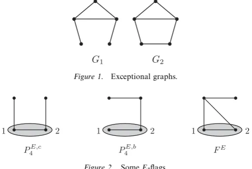
G1 G2
Figure 1. Exceptional graphs.
1 2
P4E,b
1 2
FE
1 2
P4E,c
Figure 2. SomeE-flags.
Inequality (3.6) is also used in the proof, so it has to be tight. Since we assumed that
φ0( ¯P3)>0, we have that φ0(P¯3EK3EE)>0, where ¯P3E is the uniqueE-flag on ¯P3. But
P¯E
3 K3EE=
1 4K¯1,3+
1 3P¯
(1) 3 1,
and the claim follows.
The two graphs in Figure 1, calledG1 andG2, will play a special role.
Claim 4.6. φ0(G1) =φ0(G2) = 0.
Proof. We apply the same strategy (although with much more involved calculations) as the one used to prove (4.5). Namely, we make up an analogue of (3.9) that is tight on extremal homomorphisms and such that the ‘overall slackness’ involved will coverG1
andG2.
Form the elementfE∈FE
4 as follows:
fEdef= 1 2P
E,c 4 −
1 2P
E,b 4 −FE,
whereP4E,c, P4E,b, FE ∈FE
4 are shown on Figure 2. Since (3.6) is tight,
φE0(K3E)< 1
3h
t(a) =⇒ φE0( ¯P3E) = 0 a.e.
Since both P4E,b andFE contain ¯PE
3, this implies that
φE0(K3E)< 1
3h
t(a) =⇒ φE0(fE)0 a.e. (4.6) (Recall thatht is just the restriction ofh to the interval [1−1/t,1−1/(t+ 1)] as defined
by (3.1).) Thus, by (3.3), we can multiply the left-hand side of (4.6) by fE, obtaining a
that
φ0(fEK3EE)
1 3h
t(a)φ0(fEE). (4.7)
Next, similarly to [35, (3.4)] but multiplying [35, (3.2)] (i.e., our formula (3.4) which is equality a.e.) byK1
3 rather than bye, we obtain
φ0(3(K31)21−2ht(a)eK311) =b(3b−2aht(a)). (4.8)
Subtracting (4.8) from (4.7) multiplied by 3, and re-grouping terms, we obtain
3φ0(fEK3EE−(K31)21) +ht(a)φ0(2eK311−fEE)b(2aht(a)−3b). (4.9)
But we also have
2eK311−fEE =
4 3K3+
2 3K4−
1
3K¯1,3 (4.10)
and
fEK3EE−(K31)21
1
60(G1+G2)−
1 2K4+
1 3ρK3+
1 6K5
. (4.11)
Substituting these relations into (4.9), and using Claim 4.4, we conclude by (4.5) that
1
20φ0(G1+G2)b(2ah
t(a)−3b)−ht(a)
4 3b+
2 3h
(4)(a)
+
3 2h
(4)(a) +ab+1
2h
(5)(a)
= 0.
Claim 4.6 is proved.
Lemma 4.7. Let G be a graph on V ={x1, x2, x3, y, z} with the following properties. The
verticesx1, x2, x3 induceP¯3 withx1x2 ∈E(G),y is adjacent to eachxi andzis non-adjacent to at least onexi.
Ifyz∈E(G), thenGcontainsK¯1,3 as an induced subgraph orGis isomorphic toG1orG2.
Proof. If zx1, zx2∈E(G), then zx3∈E(G) and G−y∼= ¯K1,3. If zx1, zx2∈E(G), then
G−x3∼= ¯K1,3. So we can assume without loss of generality that zx1∈E(G) and zx2 ∈
E(G). Now, ifzx3∈E(G), thenGis isomorphic toG1; otherwiseG∼=G2.
Now we are ready to put everything together. The next argument would look particularly simple and elegant in genuinely flag-algebraic notation, but it would require introducing some more notions and techniques, notably upward operators ([34, Section 2.3.1]) and relating extensions for different types ([34, Theorem 3.17]). We prefer not to indulge into this endeavour in the concluding part of our paper, so we replace this with (admittedly, crude) translation to the finite world.
Let σ be the 3-vertex type whose graph is ¯P3 with labels 1 and 2 being adjacent. Let
{Gn}converge toφ0with|V(Gn)|=n. By Claim 4.5,Gnhas Ω(n4) copies ofF0∈F40, which