warwick.ac.uk/lib-publications
Manuscript version: Author’s Accepted Manuscript
The version presented in WRAP is the author’s accepted manuscript and may differ from the
published version or Version of Record.
Persistent WRAP URL:
http://wrap.warwick.ac.uk/105492
How to cite:
Please refer to published version for the most recent bibliographic citation information.
If a published version is known of, the repository item page linked to above, will contain
details on accessing it.
Copyright and reuse:
The Warwick Research Archive Portal (WRAP) makes this work by researchers of the
University of Warwick available open access under the following conditions.
Copyright © and all moral rights to the version of the paper presented here belong to the
individual author(s) and/or other copyright owners. To the extent reasonable and
practicable the material made available in WRAP has been checked for eligibility before
being made available.
Copies of full items can be used for personal research or study, educational, or not-for-profit
purposes without prior permission or charge. Provided that the authors, title and full
bibliographic details are credited, a hyperlink and/or URL is given for the original metadata
page and the content is not changed in any way.
Publisher’s statement:
Please refer to the repository item page, publisher’s statement section, for further
information.
Flux-driven and geometry-controlled spin filtering for arbitrary spins
in aperiodic quantum networks
Amrita Mukherjee,1,*Arunava Chakrabarti,1,†and Rudolf A. Römer2,‡
1Department of Physics, University of Kalyani, Kalyani, West Bengal-741 235, India
2Department of Physics and Centre for Scientific Computing, University of Warwick, Coventry CV4 7AL, United Kingdom
(Received 6 March 2018; revised manuscript received 11 May 2018; published 13 August 2018)
We demonstrate that an aperiodic array of certain quantum networks comprising magnetic and nonmagnetic atoms can act as perfect spin filters for particles with arbitrary spin state. This can be achieved by introducing minimal quasi-one dimensionality in the basic structural units building up the array, along with an appropriate tuning of the potential of the nonmagnetic atoms, the tunnel hopping integral between the nonmagnetic atoms, and the backbone, and, in some cases, by tuning an external magnetic field. This latter result opens up the interesting possibility of designing a flux-controlledspin demultiplexerusing quantum networks. The proposed networks have close resemblance with a family of recently developed photonic lattices, and the scheme for spin filtering can thus be linked, in principle, to the possibility of suppressing any one of the two states of polarization of a single photon, almost at will. We use transfer matrices and a real space renormalization group scheme to unravel the conditions under which any aperiodic arrangement of such topologically different structures will filter out any given spin projection. The filtering turns out to be engineered by an energy-independent commutation of the basic transfer matrices, which results out of a unique set of correlation between the system parameters and/or the external flux. The commutation generates absolutely continuous subbands populated by extended, Bloch-like eigenstates in the densities of states, even for such aperiodic systems, thus defying localization and creating unattenuated transport over a continuous range of energy eigenvalues. This is an example which goes well beyond the previous studies on disordered systems, where delocalization of single particle excitations could be achieved by resonance, but only for a finite set of energy eigenvalues of the system. Our results are analytically exact, and corroborated by extensive numerical calculations of the spin-polarized transmission and the density of states of such systems.
DOI:10.1103/PhysRevB.98.075415
I. INTRODUCTION
Spintronics is all about implementing the idea of transport-ing information through the electron’s spin instead of its charge [1–3]. Naturally, the need to gain a comprehensive control over the prospect of filtering out one component (projection) of the two spin states of an electron and generating a spin-polarized current turns out to be an important issue in developing spintronic devices [4]. Experiments, beginning a couple of decades ago, exploited the quantum confinement of electrons [5,6], and the tunability of spin filters in GaAs samples was studied in detail [7]. The development of a quantum spin pump using a GaAs quantum dot (QD) [8], and spin-polarized transport studies in magnetic nanowires [9] ushered new light into this exciting research arena. One should also mention molecular wires and spin-polarized tunneling device [10], which were also examined before as potential candidates to achieve spin-controlled transport.
The experiments inspired a lot of theoretical investigations that revealed interesting properties related to spin transport and filtering in quantum devices. These systems do not remain far from being realized in real life, thanks to the immense
advance-*[email protected] †[email protected] ‡[email protected]
ment in lithography and nanotechnology. To name a few such theoretical studies, spin filtering and complete localization effect in a QD network [11], or the interplay of Rashba spin-orbit interaction (RSO) and an external magnetic field, leading to a spin-filtering effect in a QD network [12,13], were among the earlier investigations. Spin-polarized coherent electronic transport in-low dimensional networks of QDs or magnetic nanowires [14–18], or the study of a silicine nanoribbon [19] and spin filtering in an engineered graphene nano-ribbon [20] enrich the recent literature, revealing many subtleties in spin-polarized quantum transport. The interesting effect of an inhomogeneous magnetic field on the spin-dependent conductance and a filtering effect in mesoscopic ring structures was also investigated in detail [21]. Some other works in this area involve a Keldysh nonequilibrium Green’s function formalism to study spin-current production in hybrid T-shaped devices [22], spin transport in a periodic array of QD rings [23], and a study of transport through a double QD molecule [24].
Many of the network devices (NDs) modeled as described above have single or multiple loop structures providing a variety of quantum interference effects which are crucial in designing spin filters. Even in simple forms, the NDs, described within a tight binding framework and without consideration of the RSO interaction, have been shown to lead to spin-filtering effects [25].
a spin filter for higher spins by engineering the substrate, composed of a periodic array of magnetic atoms, was proposed and analysed in detail [26]. To the best of our knowledge, no results exist which explore the possibility of observing spin-polarized transport of a projectile with spins1/2, when the underlying lattice structure (the ND) is no longer periodic. To put the issue in a much more direct way, one can simply ask if disorder, which leads to localization of all the single particle states [27], rules out the possibility of spin filtering in a ND. In addition to this, another pertinent question is the role of local topology of the atomic clusters of the ND and the tunability of spin-polarized transport by an external agent such as a magnetic field. This paper is our first step to resolve such issues.
We find interesting results. In the first few examples, it is observed that, if a projectile with spins1/2 travels through a ND constructed as anaperiodicarray of atomic clusters with a short range hopping, it is very much possible to filter out justonespin channel out of the available number of (2s+1), blocking the others. This can be achieved by forming the ND as an essentially linear chain of magnetic atoms, with a set of nonmagnetic atoms attached from one side. The system thus attains a quasi-one dimensionality, but at a minimal level. The nonmagnetic QDs have to have their on-site potentials tuned to special values, for example, by a gate voltage, to initiate the spin-filtering effect. The “special” value of this potential can be calculated exactly. In addition, we show that in certain cases, such filtering can be effected only if the hopping integrals along different branches of the ND have a definite correlation between their numerical values. In a second set of examples, we show how, with a prefixed set of values of the parameters of the tight binding Hamiltonian, a wide class of NDs can filter out any desired spin stateonlyby tuning an external magnetic flux threading the plaquettes of the ND. This tempts us to propose a flux-controlledspin demultiplexerin such low-dimensional systems.
It turns out that the spin-polarized transport in such aperi-odic, quasi–one-dimensional quantum networks is intimately connected to a complete delocalization of the single particle states under certainresonanceconditions, subtle and unusual. This is a nontrivial variation of the canonical case of An-derson localization [27], which has recently been pointed out in the literature [28–30], and plays a crucial role in this analysis.
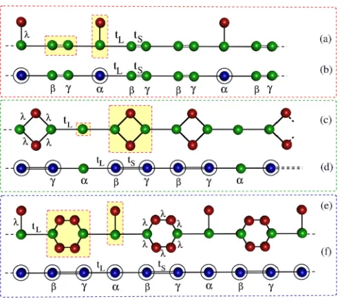
[image:3.590.302.549.58.275.2]Quite interestingly, one can identify some of the geometries we discuss in this paper, and shown in Fig. 1, with those developed in recent times in the field of photonics [31–33]. Femtosecond laser writing techniques allow one to build, experimentally, “lattices” for light, and that too in various ge-ometries. In scalar-paraxial approximation, the propagation of light in such photonic lattices is governed by a Schrödinger type equation [32]. Comprehensive control can now be achieved over the “intersite” tunneling and the “on-site” potentials. This makes these systems an ideal test bed for the study of problems related to localization and generation of flat, nondispersive bands in photonic systems, much in the spirit of dealing with spinless fermions on a lattice. It is thus tempting to conjecture that the controlled filtering of one spin projection for a “spin-half” projectile may inspire the idea of suppressing any one of the two states of polarization of a single photon.
FIG. 1. Three examples of quasiperiodic Fibonacci sequence of quantum network units with different geometries are depicted in (a), (c), and (e). The basic building blocks (highlighted) in each array consist of magnetic (green) sitting on the backbone, and nonmagnetic (red) atoms coupled to them from one side, as shown. (b), (d), and (f) represent the effective linear chains that are obtained by renormalization of the structural units, as explained in the text.
The results we obtain in this communication are valid irrespective of the geometrical nature of the array of the NDs. However, here we present results specifically for a quasiperiodic geometry, viz., NDs in a Fibonacci sequence, which allows us to extract analytically exact results. In Sec.II, we chalk out the scheme of the analysis and, in Sec.III, the results are presented without and with a magnetic field through the plaquettes. We conclude in Sec.V.
II. THE MODEL AND THE BASIC EQUATIONS
Let us refer to the set of ND geometries depicted in Fig.1. We first explain the scheme in terms of the simplest looking system, which is Fig. 1(a), henceforth referred to as the dot-stub chain. It’s an electronic counterpart of a similar dot-dot-stub photonic lattice, that was fabricated by laser inscription and investigated by Realet al.[31] who demonstrated there that the trapped photonic modes in phase coherent superpositions lead to all optical logic gate operations. In the spin-filtering problem discussed here, a sequence of magnetic atoms is arranged in a quasiperiodic Fibonacci sequence. We have two kinds of
bonds, namely,L(for “long,” say) andS(for “short”), marked
by a “double” bond. The chain grows following the well-known Fibonacci inflation ruleL→LSandS→L, and begins with anLbond. We work within a tight-binding formalism, and the Hamiltonian is given by
H=
n
cn†(n−hn·sn)cn+
n,m
(cn†tn,mcm+H.c.), (1)
In the above, each of the operatorsc†n andcn, is a single column or row with the number of entries depending on the spin component. For example, for a spin-half particle, the creation (annihilation) operatorc†n(cn), the on-site energy matrix n, and the nearest-neighbor hopping matrixtn,mare
cn†=
c†n,↑ c†n,↓
, cn=
cn,↑ cn,↓
,
n=
n,↑ 0 0 n,↓
, tn,m=
tn,m 0 0 tn,m
. (2)
The term hn·sn(s) =hn,xsn,x(s) +hn,ysn,y(s) +hn,zsn,z(s) in Eq. (1) describes the interaction of the spin (s) of the incoming projectile with the localized on-site magnetic momenthnat siten. For spin-half, the explicit form ofhn·s(ns)in terms of a matrix representation is given by [26]
hn·s1n/2=
hncosθn hnsinθne−iφn hnsinθneiφn −hncosθn
, (3)
wherehn,θn, andφnrepresent the radial component and the polar and azimuthal angles, respectively.
The Fibonacci arrangement of the bonds requires separate nomenclature for the on-site potentials. We assign the names as follows. The site flanked by anLLpair is namedα, while the sites sitting in between anLSand anSLpair of bond are named β and γ, respectively. There is a single level nonmagnetic QD [cf. Fig.1(a)] attached from one side to everyα vertex. The tunnel hopping integral between the dot and the backbone is termedλ. In the analysis that follows, we set the on-site potential at each site on the backbone asα,σ =β,σ =γ ,σ = , for every spin projectionσ. Its understandable thatσ =1/2 (↑), or−1/2 (↓) in the spin-half case, while,σ =1, 0 and−1 for a particle with total spins=1, and so on. The side-coupled QDs in Figs. 1(a), 1(c), and 1(e) are nonmagnetic in nature, and are assigned a potentialN, that can be tuned by a gate voltage. The strength of the magnetic moment (equivalently, the “local field”)hncan, in principle, assume three different values, viz., hα,hβ, andhγfor theα,β, andγsites, respectively, depending on the chemical species of the atoms employed. For simplicity, we choosehα =hβ=hγ =hin what follows here.
We calculate transmission properties for different spin channels using the standard transfer matrix method, assuming that two semi-infinite, perfectly periodic, and nonmagnetic leads connect the system at its left and the tight ends. The leads are described by a tight-binding Hamiltonian, and have on-site potentiallead, and nearest-neighbor hopping integral
tlead. The method is discussed in further detail elsewhere [26].
III. SPIN FILTERING WITHOUT EXTERNAL MAGNETIC FIELD
A. The spin-half case and the dot-stub geometry
To explain the basic scheme, we choose the dot-stub geom-etry in Fig.1(a), and the spin-half case at the beginning. We chooseθn=φn=0 to first unravel the spin-filtering properties in a completely analytical way. We begin by decimating the amplitude of the wave function at every nonmagnetic site, in terms of the amplitude at theαsite at its base. Once this is accomplished, the amplitude of the wave function at site
n, lying entirely on the backbone, satisfies the Schrödinger equation H=E, with =n,σψn,σ|n, σ, and σ = ±1/2, written in an equivalent “difference equation” form as [26]
E−
−2σ h+ λ
2
E−N
ψn,σ =tLψn−1,σ+tLψn+1,σ,
[E−(−2σ h)]ψn,σ =tLψn−1,σ+tSψn+1,σ,
[E−(−2σ h)]ψn,σ =tSψn−1,σ+tLψn+1,σ, (4)
for α, β, and γ sites, respectively, and the on-site energy at the nonmagnetic sites is denoted by N. It is interesting to note that this seemingly trivial one-dimensional backbone has the flavor of an extra or synthetic dimension hidden in it, which unfolds only to the incoming projectile depending on its spin state s. The array of magnetic atoms appears as a (2s+1)-strandladder networkto a projectile with spins [26]. Incidentally, similar multistrand ladder networks (MLN) in tight-binding formalism have previously been explored as prototypes of DNA molecules, with the interarm “cross hoppings” along the diagonals [34] simulated here by the terms hnsinθne±iφn in Eq. (3), in respect of their device aspects or charge transportation [35,36]. Some other studies involving similar MLNs include the issue of delocalization of single particle states in properly engineered disordered or aperiodic quantum networks [37,38].
B. Engineering a spin filter
Equation (4) is actually a set of six equations, grouped in two subsets. Each subset, consisting of three equations, represents two decoupled, independent Fibonacci chains. In each subset, the first equation is written for anαsite, while the two subsequent equations are written for the sites of typeβ andγ, respectively. Theα-site potentials for the↑and↓spin projections for the two decoupled Fibonacci chains are given, respectively, by
˜
α,σ =−2σ h+ λ2
E−N
, (5)
while for theβandγsites these are ˜β,σ =˜γ ,σ =−2σ h. A pertinent issue to discuss here is the role of the “local” magnetic field h offered by the magnetic atoms on the backbone. A large value ofh will naturally split the bands for the↑and the↓ spins [26]. Therefore, even when λ=0, that is, when we have a purely one dimensional Fibonacci lattice, the ↑ and↓ spins will have their spectra separated on the energy scale. Each such spectrum will have the usual three subband structure [39]. The transport for the two spin projections will be there, over these two energy regimes, exhibiting the usual multifractal character [39], thinning out as the system attains its thermodynamic limit. Spins will still get filtered out, but in a scanty, fractal way. Most importantly, due to the Cantor set character of the energy spectrum, it is impossible to locate an energy eigenvalue exactly for an infinite system.
for↑and↓spins at appropriately chosen domains over the full spectral zone. Let us look at Fig.1(b). On this effectively one-dimensional Fibonacci chain, we find two distinct “building blocks,” viz., an isolatedαsite (with renormalized potential) and a “dimer” βγ, arranged following a Fibonacci pattern. This, of course, is a generic feature of the Fibonacci lattice grown following the rule stated earlier, and thus remains valid for all the quasi-one-dimensional quantum networks discussed in this paper.
Corresponding to two such building blocks, one can construct 2×2 unimodular “transfer matrices” Mα,σ and Mγ β,σ ≡Mγ ,σMβ,σ that are given by
Mα,σ =
(E−˜α,σ)/tL −1
1 0
,
Mγ β,σ =
(E−˜γ ,σ)(E−˜β,σ) tLtS −
tS tL −
E−˜γ ,σ tS E−β,σ˜
tS −
tL tS
. (6)
The on-site potentials, viz., ˜α, ˜β, or ˜γassume their appropri-ate values depending on the spin projection, as stappropri-ated earlier.
For each spin stateσ, the pair of the amplitudes of the wave function at anyn+1th andnth sites on the linear backbone is related to any arbitrary pair of sites, marked as 1 and 0, for example, through a simple product of 2×2 transfer matrices
ψn+1,σ ψn,σ
=Mn,σ·Mn−1,σ·. . .·M2,σ·M1,σ
ψ1,σ ψ0,σ
.
(7)
Let us now work out how to transmit the↑spin for example. We choose the first subset from Eq. (4) corresponding to the↑ spin projection, and compute the commutator [Mα,↑,Mγ β,↑].
The commutator reads
[Mα,↑,Mγ β,↑]= −
(E−N)
tS2−tL2−λ2(E−+h) (E−N)tLtS
×
0 1
1 0
. (8)
It is easily verified that, if we setλ=
t2
S−tL2, andN=− h, then [Mα,↑,Mγ β,↑]=0,independent of energy. Therefore, in the chosen subset of Eq. (4) that corresponds to the↑spin case, the specific order of arrangement of the pair of sites βγ, and the isolated (stubbed) site αbecomes unimportant. Thus, we can, under this “resonance condition,” think of the Fibonacci array for the↑electrons as being composed of two
infinitely long periodic lattices, one made up of the α-sites
stubbed with the dots only, and the other, of the pairsβγ, as shown in Fig. 2. As a result, one expects a complete transparency in the transport of ↑ electrons over the range of energyE which spans the absolutely continuous spectra offered by these two periodic lattices.
It is essential to appreciate that the commutation of the matrices renders the spectrum for one of the spin states
absolutely continuous, ensuring a complete transparency over
the full energy regime. This is in contrast to the earlier case of say, the “random dimer model” [40], where transparency could be achieved only at one special value of the energy of the electron. In any generalization of the RDM, the extended
FIG. 2. (a) The periodic, infinitely long βγ dimer (shown in dotted box) lattice and (b) The infinite periodic array of the “stubbed”
αsites. The on site potentials are,α=β=γ =N=∓hfor the↑and↓spins. The vertical “tunnel” hopping in (b) is chosen as
λ=t2
S−tL2for the matrices to commute. The densities of states for these two lattices merge as the commutation of the transfer matrices is enforced. The colors are as in Fig.1.
states and complete transparency came up only at a discrete set of energy eigenvalues.
A second important point needs to be emphasized here. Each of the two linear periodic lattices in Fig.2displays two absolutely continuous subbands in their respective densities of states (DOS), which occupy different intervals of energyE. As the transfer matrices commute under the special correlations between the potentials and the hopping integrals, as stated above, these two different DOS have to merge, and have to become indistinguishable from the DOS of the Fibonacci array of stubbedαsites and theβγ dimers. Otherwise, the energy interval over which the↑spins will be filtered out is going to be ill defined, and the scheme of spin filtering should not work. We have checked this analytically by calculating the local DOS ρβ,↑ at the β or ργ ,↑ at the γ site of the first chain (the periodic βγ array, withρβ,↑=ργ↑), andρα,↑ at theα site of the remaining chain. This gives us an estimate of the band positions and the widths in the two cases. We have set, for simplicity of the expressions,N,↑=α,↑=β,↑ =γ ,↑= −hbeforehand. The DOSs are given by
ρβ,↑ = 1 π
E−+h
4t2
LtS2−
(E−+h)2−t2
L+tS2
2,
ρα,↑ = 1 π
E−+h
4tL2(E−+h)2−[(E−+h)2−λ2]2 . (9)
It is simple to verify from Eq. (9) thatρβ,↑=ρα,↑ as soon as we enforce
λ=
tS2−tL2. (10)
The results are similar when we choose to transport the↓spins. The selection of the potentials in this case now will bei,↓= +h, withi≡α,β,γ and the nonmagnetic dot. The choice of the tunnel hoppingλremains the same.
[image:5.590.300.551.58.134.2]variety of geometrical arrangements, periodic, quasiperiodic or random, involving the same networks exhibits complete delocalization of the eigenstates under the same conditions and in a way, group together to exhibit a subtleuniversality class. In terms of photonics, engineering apolarization filter
for photons may be given a consideration, thinking in this line. The above discussion remains valid for the two remaining geometries shown in Fig.1as well, for which the difference equations and the commutators are presented in the Appendix. Back to the filtering of the spin states, we see that the second subset in Eq. (4) still represents a quasiperiodic Fibonacci chain for the↓ spin electrons, with its own, typically multifractal DOS [39]. The complete spectrum of the system shown in Fig.1(a)is obtained from a convolution of the DOS arising out of the two subsets of Eq. (4) corresponding to the↑and↓spins. An appropriate choice of the strength of the magnetic moment hcan separate out the spectra arising out of the two subsets [26] on energy axis, thereby removing the possibility of any overlap between the absolutely continuous subbands from the↑spin equations, and the fractal spectrum contributed by the second subset; that is, for the↓spins. The↑spin subbands, absolutely continuous in character, should be completely transparent over the range of energy for whichρα(β),↑is nonzero. The↓spins give rise to a multifractal, Cantor set energy spectrum.
The↓spins get transmitted in that part of the energy range, whereρα(β),↓is nonzero. The transmission spectrum is scanty, and one should expect a usual scaling behavior, typical of the Fibonacci lattice, that drops in magnitude as the system grows to its thermodynamic limit. The aperiodic dot-stub array, (and the other ones in Fig.1) can thus act as a perfect spin filter for↑spins. Choosing the self-energy of the QD at the stub, as N =+h, we can have a prefect spin filter for the↓spins, using identical arguments already outlined.
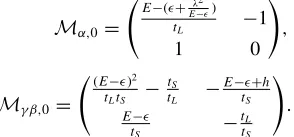
In Fig.3, we show the DOS profile and the corresponding transport characteristics of the dot-stub Fibonacci lattice. The DOS has been calculated by evaluating the matrix elements of the local Green’s function G=(E1−H)−1 for a 377 bond long lattice. The commutation conditions Eq. (10) are imposed. The ↑ spins exhibit a continuous patch of hight transmission values in the energy regime where the↑ spin subbands are absolutely continuous. On the contrary, the↓ spin shows scanty, fractal like transmission coefficients in its own “allowed” spectral zones.
C. Scheme for general spins
The formalism works perfectly well for any spin s. The “virtual” ladder we talked about before now has (2s+1) strands. If we look at the prospect of spin-polarized transport for projectiles with total spins, withθn=φn=0 as before, we have a set of (2s+1) decoupled equations. Each such set represents an independent Fibonacci chain, and is a triplet of equations, corresponding to the sites α, β, andγ as its constituents. Let us take a specific example. When the spin of the projectile iss=1, the spin projections are given byσ =1, 0, and−1. The on-site potential at anαsite in the effectively linear Fibonacci chain are ˜α,±1=∓h+λ2/(E−N), for σ = ±1, and represents the effective potential at a site of type α. Theβand theγsites are crowned with the on-site potential values ˜β,±1=γ ,±1=∓h. For the spin projectionσ =0,
(a) ρ↑
,
ρ↓
0.01 0.1 1 10
E
−6 −4 −2 0 2 4 6
(b) T↑↑
,
T↓↓
0 0.2 0.4 0.6 0.8 1
E
−6 −4 −2 0 2 4 6
FIG. 3. (a) DOS for spin-1/2 particles in the stub geometry shown in Figs.1(a)and1(b)fori=0,h=3,tL=1, andtS=2. The dashed line (with dark/blue shading) indicates the spin-up projection while the solid line (with lighter/orange shading) corresponds to the spin-down case. (b) The transmission coefficient for the same system and parameters as in (a). The dark solid (blue) line indicates spin-up while the lighter (orange) line is for spin-down. The lead parameters of the nonmagnetic leads arelead=0 andtlead=3tL.
˜
α,0=+λ2/(E−N) for anαsite, while ˜β,0 =˜γ ,0=.
The nearest-neighbor hopping integrals along the backbone remain astLortSdepending on the bonds.
Suppose we wish to filter out the spin stateσ =0. For this, we simply need to setN =. The relevant transfer matrices for σ =0 for the dot-stub case in Fig. 1(a)now assume the forms
Mα,0=
E−(+λ2 E−) tL −1
1 0
,
Mγ β,0=
(E−)2 tLtS −
tS tL −
E−+h tS E−
tS −
tL tS
. (11)
The commutator [Mα,0,Mγ β,0]=0 irrespective of the energy
[image:6.590.313.546.60.375.2] [image:6.590.354.501.580.649.2](a)
ρ1
,
ρ0
,
ρ-1
0.01 0.1 1 10
E
−10 −5 0 5 10
(b)
T11
,
T00
,
T-1-1
0 0.2 0.4 0.6 0.8 1
E
−10 −5 0 5 10
FIG. 4. (a) DOS for spin-1 particles in the stub geometry shown in Figs. 1(a) and 1(b) for i=0, h=3, tL=1, and tS=2. (b) Transmission coefficient for the stub geometry and parameters as in (a) with lead parameters of the nonmagnetic leads given bylead=0
andtlead=5tL.
σ =0 state. The selection ofN =∓h, on the other hand, allows theσ = ±1 states (only one at a time though) to tunnel through, blocking the others. In Fig.4, we present the results fors=1. With the parameter choices as above, we filter out the spin channelσ =0 as transmitting, while the other projections σ = ±1, exhibit fractal character in their DOS.
We end this section bringing an interesting variation of the proposed models to the attention of the reader. The arguments put forward so far for spin-half or spin-one, or, for any spins will hold perfectly well for a much more general situation. If the three sitesα,β, andγrepresent three chemically different species with the combinations of the on-site potentials and magnetic moments (i,σ, hi), withi≡α,β, orγ, even then we can make any desired spin channel transmit, blocking the others. For example, considering the spin-half situation, and a target of filtering out the↑spin again, we need to enforce a correlationN=i,σ−hi =a constant. One can now afford to take the individual values ofi andhi even from a set of random numbers, but always maintaining the above correlation in their numerical values. The tunnel hopping integralλstill
should be chosen as
[image:7.590.301.549.58.280.2]
tS2−tL2. The matrices will commute, and we shall have the liberty to engineer a spin filter even now. Same arguments remain valid for any spin states, and for any
FIG. 5. Geometries where magnetic flux plays a pivotal role in spin filtering. (a) A Fibonacci array of triangles and dots and (b) its renormalized version. (c) A Fibonacci array of diamond-shaped plaquettes and stubs, and (d) its effective renormalized one dimensional version. (e) and (f) depict the diamond-stub system and the renormalized chain, respectively. The colors are chosen as in Fig.1.
desired spin projectionσ. The scheme thus goes well beyond a quasiperiodic Fibonacci ordering and encompasses a larger canvas ofdisorderedsystems as well.
IV. SPIN FILTERING TRIGGERED BY AN EXTERNAL MAGNETIC FIELD
A. A quasiperiodic triangle-dot array
We now have a look at lattices shown in Fig.5. To gain an insight, let us focus on the simplest of them, viz., Fig.5(a), a quasiperiodic triangle-dot array, and its renormalized ver-sion which is the effective one dimenver-sional Fibonacci chain shown in Fig. 5(b). In the array of triangles and dots, a uniform magnetic flux threads each triangular plaquette. The corresponding magnetic field points, say, in the positive zdirection. The hopping integral along an arm of the triangle is designated byλ, and it now carries a “Peierls” phase with it. The phase factor is±exp(2π i/30)between the vertices
of the triangle,being the flux “trapped” in the triangle, and 0=hc/ebeing the flux quantum. The “triangle-dot” array
presents a system where the time-reversal symmetry is broken, but only partially, as the particle hops along the edges of the triangle. The on-site potentials of the effectiveβandγsites on the linear backbone becomeβ,σ =γ ,σ =+λ2/(E−N) on decimating the nonmagnetic vertices.
tSF(B) ≡tβ(γ)→γ(β), are now given bytSF(B)=tSe±iη, where
tS =
λ2+ λ 4
(E−N)2
+ 2λ3 E−N
cos
2π
0
, (12)
tanη= (E−N) sin−λsin 2 (E−N) cos+λcos 2
. (13)
Here,=2π/(30).
Let us explain the spirit of spin filtering in this case in terms of a spin-half projectile, just as we did before. The remaining spins can be analyzed following the scheme discussed in the last section. The Fibonacci array is, as before, composed of two bonds, characterized by the hopping integrals tL and tSexp±iη, along which the time-reversal symmetry is broken. The decoupled set of equations for θn=φn=0, and σ = ±1/2, respectively, are now
[E−(−2σ h)]ψn,σ =tLψn−1,σ +tLψn+1,σ,
E−
−2σ h+ λ
2
E−N
ψn,σ =tLψn−1,σ
+tSeiηψn+1,σ,
E−
−2σ h+ λ
2
E−N
ψn,σ =tSe−iηψn−1,σ
+tLψn+1,σ.
(14)
for theα,β, andγsites, respectively.
Following the reasoning given before, let us choose the first subset of these equations, and setN =−h (for↑ spins). The commutator [Mα,↑,Mγ β,↑] reads
[Mα,↑,Mγ β,↑]
=e
4π i30
tL2−2λ2(E−+h)−2λ3cos
2π 0
λtL[e2π i
0(E−+h)+λ]
×
0 1
1 0
. (15)
The commutator is seen to vanish irrespective of energy for λ=tL/
√
2, and for amagnetic flux=0/4. The spectrum
consists of absolutely continuous subbands, for the ↑ spins only. The transport for the↑spins remains perfect and unat-tenuated in these parts of the spectrum. The DOS for the↓spins exhibit the fragmented structure. The↓spins exhibit very weak transport in the energy regime where the↓spin band presents the scanty, fragmented, typical Fibonacci-like spectrum.
The reasoning holds perfectly well for any general spin projectionσ, as before. The combination ofλ=tL/
√ 2 and =0/4 allows just one spin channel out of the available
(2s+1) channels, blocking the others. Of course, with a general spin projectionσ, one needs to gate the potentialN appropriately, depending on which spin channel one wants to filter out. Furthermore, we note that the condition=0/4
follows from having the effective hopping, i.e., across the decimated loops enclosing the flux , be independent of a phase difference between clockwise and counterclockwise propagation.
(a)
ρ↑
,
ρ↓
0.01 0.1 1 10
E
−6 −4 −2 0 2 4 6
(b)
T↑↑
,
T↓↓
0 0.2 0.4 0.6 0.8 1
E
−6 −4 −2 0 2 4 6
FIG. 6. (a) DOS for spin-1/2 particles in the triangle-dot geome-try shown in Figs.5(a)and5(b)fori=0,h=3,tL=1,λ=tL/
√ 2 and additional magnetic flux=0/4. Colors distinguishing spin-↑
and -↓are as in Fig.3. (b) Transmission coefficient for the triangle geometry and parameters as in (a) with lead parameters of the nonmagnetic leads given bylead=0 andtlead=3tL.
In Fig.6(a), we show the DOS for the↑and the↓spins, and the corresponding transmission coefficients in Fig.6(b)when the conditions for commutation of the matrices is fulfilled. As expected, the transmission coefficient for the↑spins is high and continuously distributed precisely spanning the absolutely continuous band for the↑spins, shown in Fig.6(a). A single spike of the↓spin DOS is located around the middle for the ↑spin DOS. However, extended and localized states cannot coexist at the same energy, and in the convolved DOS of the full system, the state becomes perfectly extended. This is confirmed by the plot of the transmission coefficients in Fig.6(b).
B. The diamond-stub array
In Fig. 5, we present a few prototype systems among a variety of networks that exhibit spin filtering under the influence of an external magnetic field. While Figs.5(a)and
[image:8.590.307.551.58.389.2] [image:8.590.40.292.61.155.2]including the hopping along the arms of the diamonds. We choose to discuss it explicitly, presenting the commutator for Fig.5(c)in the Appendix. It may be mentioned that a similar diamond quantum network, but without the stubs, in a periodic array was considered recently to study the spin-polarized transport within a tight-binding framework [41]. Furthermore, we have also investigated more complex situations in which the flux-enclosing loop contains more sites than the maximally four shown in Fig. 5. In all such situations, a similar spin-filtering effect can be found.
Let us fixN=−h, keeping in mind that we are interested in filtering out the↑spin fors=1/2. In addition, we setλ= tL. On decimating the nonmagnetic vertices in Fig.5(e), the so-called short hopping in the resulting Fibonacci chain becomes equal totS=2tL2cos(π/0)/(E−N). The spin filtering can be effected in this case bytuning the external magnetic field
alonethreading every diamond plaquette. This can be quite
interesting from the standpoint of an experiment. We provide the commutation conditions for Fig. 5(c) in Appendix, and give the explicit results for the last case, which is the so-called diamond-stub case, as presented in Fig.5(e). The commutation of the matrices, once again, talking in terms of the ↑ spin filtering in the spin-1/2 case is given by
[Mα,↑,Mγ β,↑]= − tLcos
2π 0
sec
π 0
E−+h
0 1
1 0
.
(16)
It is easily seen that, the commutator vanishes for=0/4.
It is equally important to ensure again that, as the com-mutation condition is satisfied, the spectrum of a periodic array of diamonds—equivalent to the array of aβγ doublet in Fig.5(f)—and the spectrum of a periodic array of theαsites merge. In this way, one gets a perfect spin filter over a unique span of energy for the↑or the↓spins. The range of energy, of course, depends on whether we setN =−h, or+h. We have checked it in this case also. Let us write, forN =−h, the local DOS for a periodicα-chain asρα,↑ =1/(π
√
Q1), and
that of a periodic chain ofβγ doublet asρβγ ,↑ =1/(π √
Q2). It is easy to work out that the difference≡Q1−Q2is given by
= 4tL4F(E,)
(E−+h)2(E−+h)2−2t2
L
2cos
2π
0
,
(17)
where,F(E,)=E3[E−4(−h)]+(−h)2[(−h)2−
3t2
L]+2tL4+3E2[2(−h)2−tL2]+2E(−h)[3tL2−2(− h)2]−t4
Lcos(2π/0). It is clearly observed that, as soon as
we set=0/4, the differencebecomes equal to zero, and
the DOS merge. This happens for all the geometries discussed in this work, if we include the appropriate correlations in the numerical values of the potentials and the hopping elements λandt, where applicable. The summary is, if we fix the dot potential N =∓h at the very outset, then a perfect spin filter for the↑or the↓spin electrons can be achieved by tuning the magnetic flux alone. Needless to say, that the scheme works equally well for any arbitrary spins. The appropriate selection ofN will have to be made at the beginning of the
experiment. The rest can be achieved simply by tuning the flux.
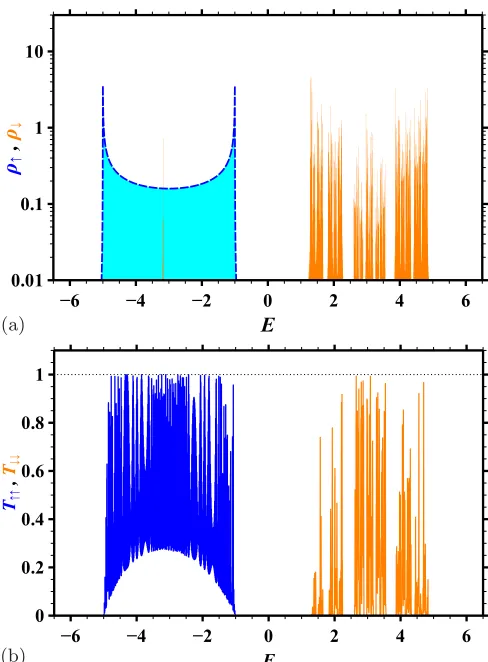
The DOS and the transmission coefficients for the↑and↓ spins in the spin-1/2 case are shown in Fig.7in four panels. For comparison, we show the “of-resonance” condition, with= 0, and the “resonance” condition with=0/4 in separate
pairs of panels Figs. 7(a)and7(b), and Figs. 7(c)and7(d), respectively. The transmission coefficientT↑,↑for the↑spin retains the fractal distribution, while the↓spins are practically forbidden even in a 377-bond-long lattice. With =0/4,
the transmission of the↓spins is totally blocked, as is evident from Fig.7(d).
V. CONCLUSIONS
We have analyzed the prospect of filtering out any arbitrary spin state and letting it tunnel through an infinitely long array of quasi-one-dimensionalquantum networks, arranged in an aperiodic fashion. The scheme relies on the commutation of the transfer matrices corresponding to the elemental building blocks of the ND. Such a commutation takes place independent of energy once we set the desired correlation between the system parameters. Since the transfer matrices commute, the scheme remains valid for any random or deterministically disordered arrangement of the network units. It has been discussed how the subtle, hidden dimensions, (2s+1) in number, opens up to an incoming particle of spin s. This is exploited in engineering the spin filter. The correlations between the values of the potential and the tunnel-hopping integrals needed to filter out a specific spin channel for all
energies, and blocking the other channels, are discussed in
detail. In another set of lattice structures, it has been discussed how a spin filtering effect can be observed by using an external magnetic field alone. The commutation of the matrices and, consequently, the existence of absolutely continuous spectrum, have been tested to be quite robust against a possible fluctuation from the exact resonance condition [28,29]. This last issue may present an interesting experimental challenge in terms of novel spin-controlled devices. The method outlined here is likely to be applicable to some photonic structures, developed recently using ultrafast laser inscription [33]. One can thus look forward to engineer a “polarization filter” for photons even.
Finally, it is worth mentioning that the results presented here are obtained within a single-band tight-binding model, and for a class of deterministic geometry. The robustness of the spin-filtering effect against random disorder has already been tested by us, and will be reported in due course. The inclusion of spin-orbit interaction or orbital hybridization is likely to play important roles in spin filtering. Work in this direction is in progress.
ACKNOWLEDGMENTS
(a) ρ↑
,
ρ↓
0.01 0.1 1 10
E
−6 −4 −2 0 2 4 6
(c) ρ↑
,
ρ↓
0.01 0.1 1 10
E
−6 −4 −2 0 2 4 6
(b) T↑↑
,
T↓↓
0 0.2 0.4 0.6 0.8 1
E
−6 −4 −2 0 2 4 6
(d) T↑↑
,
T↓↓
0 0.2 0.4 0.6 0.8 1
E
−6 −4 −2 0 2 4 6
FIG. 7. (a) DOS for spin-1/2 particles in the diamond-stub geometry shown in Figs.5(c)and5(d)fori=0,h=3,tL=1,=0. Colors distinguishing spin-↑and -↓are as in Fig.3. (b) Transmission coefficient for the diamond-stub geometry and parameters as in (a) with lead parameters of the nonmagnetic leads given bylead=0 andtlead=3tL. (c) and (d) show similar results as in (a) and (b), respectively, but now for external flux at=0/4.
Illuminating conversation with Sebabrata Mukherjee is thank-fully acknowledged. UK research data statement: All data accompanying this publication are directly available within the publication.
APPENDIX A: FIBONACCI SEQUENCE
A Fibonacci array of two lettersLandStypically represents an idealized version of a quasicrystal [42] in one dimension. The chain grows following the inflation rulesL→LS and S→L, and beginning with anL, which one may call the “first generation” G1. The subsequent generations are G2=LS,
G3=LSL, G4 =LSLLS, G5=LSLLSLSL, and so on. The infinite quasiperiodic chain can be constructed recursively, using thenth generation block Gn. Such a lattice is termed as thenthrational approximantof the true Fibonacci chain. Naturally, the true infinite quasiperiodic chain is generated as one considers the limitn→ ∞.
The standard results for excitation spectrum on a Fibonacci quasicrystals are usually obtained by describing the system in terms of an array of two “bonds”LandS. The tight-binding description needs identification of two kinds of “hopping integrals,”tL andtS, and three kinds of atomic sites marked by the on-site potentialsα,β, andγ assigned to the vertices residing between anLL pair or anLS pair or an SL pair, respectively. It is convenient to introduce transfer matrices Mα,Mα, andMγ. The matricesMαandMγ β=Mγ.Mβ resemble the ones written down, for example, in Eq. (6). The
string of the transfer matrices for a recursively grown Fibonacci sequence, built using thenth generation rational approximant Gn, follow the growth rule
MGn=MGn−2MGn−1. (A1)
The energy spectrum is obtained using the so-called trace map [43], viz.,
xn=2xn−1xn−2−xn−3, (n4), (A2)
where xn=(1/2) Tr[MGn]. The first three values x1= Tr[Mα]/2, x2=Tr[Mγ β]/2, and x3=Tr[Mα.Mγ β]/2. The rest follows easily from Eq. (A2). The allowed eigenvalues are those for whichxn1. The energy spectrum, in general, turns out to be a Cantor set, with measure zero, and the wave functions exhibit a multifractal character [44].
APPENDIX B: DIAMONDS AND DOTS AT ZERO FLUX
We refer to Figs.1(c)and1(d). On the renormalized lattice Fig.1(d), the on-site potentials for the spin-half case, and the hopping integrals are given by
α,σ =−2σ h,
β,σ =γ ,σ =−2σ h+ 2λ2 E−N
. (B1)
[image:10.590.87.510.58.336.2]tS=2λ2/(E−N). The difference equations read
[E−(−2σ h)]ψn,σ =tLψn−1,σ +tLψn+1,σ,
E−
−2σ h+ 2λ
2
E−N
ψn,σ =tLψn−1,σ +tSψn+1,σ,
E−
−2σ h+ 2λ
2
E−N
ψn,σ =tSψn−1,σ +tLψn+1,σ.
(B2) In each set the sequence of equations, from top to bottom, represents theα,β, and theγ sites, respectively.
The transfer matricesMα,↑andMγ β,↑ ≡Mγ ,↑Mβ,↑can now easily be constructed following the old prescription, and the commutator, for the↑spin, for example, becomes
[Mα,↑,Mγ β,↑]=
EtL2−2λ2+2λ2(−h)−NtL2 2tLλ2
× 0 1 1 0 . (B3)
The off-diagonal elements, and hence the entire commutator vanishes forλ=tL/
√
2, andN=−h.
APPENDIX C: HEXAGON AND STUB IN ZERO FLUX
This geometry needs all the nearest-neighbor hopping integrals to be identical to see the desired spin filtering effects. We take every nearest-neighbor hopping integral along the backbone, including the arms of the hexagon and the backbone—stub atom tunnel-hoppingλequal totL. For spin projection σ, on renormalization the on-site potentials and the hopping integrals along the effective one-dimensional Fibonacci chain in Fig.1(f)read
α,σ =−2σ h+ t2
L E−N
,
β,σ =γ ,σ =−2σ h+
2(E−N)tL2 (E−N)2−tL2
,
tS =
2t3
L (E−N)2−tL2
. (C1)
The commutator that we are interested in reads
[Mα,↑,Mγ β,↑]=
(−h−N) 2t2
L(E−N)
(E−N)2+tL2
× 0 1 1 0 , (C2)
which clearly vanishes as we setN=−h.
APPENDIX D: THE ARRAY OF SQUARE NETWORKS THREADED BY A MAGNETIC FLUX
We now provide with the commutator for the geometry depicted in Fig.5(b). The squares can stand isolated as well as touch each other, as shown. The other cases, including any general spinssituation, can be worked out easily.
The effective on-site potentials and the hopping integrals, for a spin projectionσ(= ±1/2) are given by
˜
α,σ =−2σ h+
2λ2(E−
N) (E−N)2−λ2
,
˜
β,σ =˜γ ,σ =−2σ h+
λ2(E−
N) (E−N)2−λ2
,
tLF =λei+ λ
3e−3i
(E−N)2−λ2
. (D1)
Here,=π/20. The double bonds are the “short” bonds
in our description of a Fibonacci sequence, and has the hopping integral tS associated with it, while the hopping along the “long” bonds is now associated with a phase, as is obvious from Eq. (D1).
For the↑spin, the construction of the matricesMα,↑and Mγ β,↑ ≡Mγ ,↑Mβ,↑ are now straightforward. To simplify matters, let us presetN =−h. The commutator, for a given set of values oftS,andh, andσ =1/2 now reads
[Mα,↑,Mγ β,↑]=ξ
0 m12
m21 0
, (D2)
where
ξ =2λ4cos
2π
0
+tS2−2λ2[λ2−(E−+h)2],
(D3)
and
m12=e3π i 20
(E−+h)2e−iπ0 +
2iλ2sinπ 0
λtS
2iλ2sinπ 0
+eπ i0(E−+h)22
,
m21=
−e−π i20 λtS
2iλ2sinπ 0
−eπ i0(E−+h)2
. (D4)
It is easy to see thatξ =0 forλ=tS/ √
2, and=0/4;
the commutator vanishes identically.
[1] G. A. Prinz,Phys. Today48(4),58(1995). [2] G. A. Prinz,Science282,1660(1998). [3] S. A. Wolf,Science294,1488(2001). [4] S. Murakami,Science301,1348(2003).
[5] D. Goldhaber-Gordon, H. Shtrikman, D. Mahalu, D. Abusch-Magder, U. Meirav, and M. A. Kastner,Nature391,156(1998). [6] S. M. Cronenwett, T. H. Oosterkamp, and L. P. Kouwenhoven,
Science281,540(1998).
[7] L. P. Rokhinson, V. Larkina, Y. B. Lyanda-Geller, L. N. Pfeiffer, and K. W. West,Phys. Rev. Lett.93,146601(2004).
[8] S. K. Watson, R. M. Potok, C. M. Marcus, and V. Umansky, Phys. Rev. Lett. 91, 258301
(2003).
[9] V. Rodrigues, J. Bettini, P. C. Silva, and D. Ugarte,Phys. Rev. Lett.91,096801(2003).
[10] R. P. Andres, T. Bein, M. Dorogi, S. Feng, J. I. Henderson, C. P. Kubiak, W. Mahoney, R. G. Osifchin, and R. Reifenberger,
Science272,1323(1996).
[11] D. Bercioux, M. Governale, V. Cataudella, and V. M. Ramaglia,
[12] A. Aharony, O. Entin-Wohlman, Y. Tokura, and S. Katsumoto,
Phys. Rev. B78,125328(2008).
[13] P. Földi, O. Kálmán, M. G. Benedict, and F. M. Peeters,Nano Lett.8,2556(2008).
[14] H.-F. Lü, S.-S. Ke, X.-T. Zu, and H.-W. Zhang,J. Appl. Phys. 109,054305(2011).
[15] R. Wang and J.-Q. Liang,Phys. Rev. B74,144302(2006). [16] A. A. Shokri, M. Mardaani, and K. Esfarjani,Phys. E:
Low-Dimensional Syst. Nanostruct.27,325(2005).
[17] M. Mardaani and A. A. Shokri,Chem. Phys.324,541(2006). [18] M. Dey, S. K. Maiti, and S. N. Karmakar,Eur. Phys. J. B80,
105(2011).
[19] C. Núñez, F. Domínguez-Adame, P. A. Orellana, L. Rosales, and R. A. Römer,2D Mater.3,025006(2016).
[20] D. Kang, B. Wang, C. Xia, and H. Li,Nanoscale Res. Lett.12,
357(2017).
[21] M. Popp, D. Frustaglia, and K. Richter,Nanotechnology14,347
(2003).
[22] I. L. Fernandes and G. G. Cabrera,Physi. E: Low-Dimensional Syst. Nanostruct.99,98(2018).
[23] X. Hai-Bin, Z. Han-Yin, N. Yi-Hang, L. Zhi-Jian, and L. Jiu-Qing,Chin. Phys. B19,047303(2010).
[24] M. L. Ladrón de Guevara, F. Claro, and P. A. Orellana,Phys. Rev. B67,195335(2003).
[25] H.-H. Fu and K.-L. Yao,J. Appl. Phys.111,124510(2012). [26] B. Pal, R. A. Römer, and A. Chakrabarti,J. Phys.: Condens.
Matter28,335301(2016).
[27] P. W. Anderson,Phys. Rev.109,1492(1958).
[28] B. Pal and A. Chakrabarti,Phys. Lett. A378,2782(2014). [29] B. Pal, S. K. Maiti, and A. Chakrabarti,Europhys. Lett.102,
17004(2013).
[30] A. Nandy, B. Pal, and A. Chakrabarti, Europhys. Lett.115,
37004(2016).
[31] B. Real, C. Cantillano, D. López-González, A. Szameit, M. Aono, M. Naruse, S. J. Kim, K. Wang, and R. A. Vicencio,
Sci. Rep.7,15085(2017).
[32] S. Mukherjee, A. Spracklen, M. Valiente, E. Andersson, P. Öhberg, N. Goldman, and R. R. Thomson,Nat. Commun. 8,
13918(2017).
[33] S. Mukherjee and R. R. Thomson, Opt. Lett. 40, 5443
(2015).
[34] C. J. Páez, P. A. Schulz, N. R. Wilson, and R. A. Römer,New J. Phys.14,093049(2012).
[35] S. A. Wells, C.-T. Shih, and R. A. Römer,Int. J. Mod. Phys. B 23,4138(2009).
[36] G. Cuniberti, E. Maciá, A. Rodríguez, and R. A. Römer,
Tight-Binding Modeling of Charge Migration in DNA Devices
(Springer, Berlin, 2007), pp. 1–20.
[37] S. Sil, S. K. Maiti, and A. Chakrabarti,Phys. Rev. Lett.101,
076803(2008).
[38] A. Rodriguez, A. Chakrabarti, and R. A. Römer,Phys. Rev. B 86,085119(2012).
[39] M. Kohmoto, B. Sutherland, and C. Tang,Phys. Rev. B35,1020
(1987).
[40] D. H. Dunlap, H.-L. Wu, and P. W. Phillips,Phys. Rev. Lett.65,
88(1990).
[41] B. Pal and P. Dutta,Sci. Rep.6,32543(2016). [42] E. Maciá,Phys. Rev. B60,10032(1999).
[43] M. Kohmoto, L. P. Kadanoff, and C. Tang,Phys. Rev. Lett.50,
1870(1983).
[44] M. Severin and R. Riklund, Phys. Rev. B 39, 10362