Predictive Vehicular Traffic Model Using Ensemble Methods

Predictive Vehicular Traffic Model Using Ensemble

Methods

Aysha Jagiasi1, Pavan Chhatpar2, Sumeet Shahani3, Nimesh Doolani4, Priya R. L5,

1, 2, 3, 4, 5

Computer Engineering, VESIT

Abstract: Traffic will always be a problem as we move to a modernized way of living. And in those stages of evolution, the complexity increases which in turn demands even more sophisticated measures to tackle them. Machine learning techniques have always helped in making efficient systems with minimal continual human intervention. A similar system is described in this paper. The data was collected from Google Maps. A processing technique was applied to extract features from the raw data. A significant amount of effort was put towards data preparation in order to make the features suitable for the proposed system. Multiple approaches to model the traffic data were tested before finalizing the model which best suited for this proposal. For this research, a few selected areas were chosen. The system built is scalable and can be expanded to cover more areas.

Keywords: Machine Learning, Data Mining, Geohash, Traffic congestion, Route generator.

I. INTRODUCTION

Traffic is a very important and unavoidable circumstance which can dampen the daily routine and its solutions need to be updated continually. Various reasons contribute to traffic. It is a wider categorisation. We have often come across bottlenecks which occur as a result of a wider road leading into a narrower one. This can lead to extension of the pile of vehicles and also occupy other lanes as well. The other reason for clogging can be improper lane changing. Considering a road with multiple civil transport vehicles and other private ones, these reasons just progressively add to traffic. At times, negligent driving leads to accidents which bring the entire stretch to a halt.

Therefore, people should have an overview of the traffic intensity before they plan their journey. They should be able to decide between taking the public transport or their own vehicles. This leads to a requirement of a system which has the ability to capture, store, and analyse the traffic intensity. Any user can be prompted and advised on regular traffic updates, which will help them to decide, in advance or during transit, on their plans or alternate routes.

Bringing autonomy in systems that assist humans in everyday tasks and adapt with their lifestyle is one of the grand challenges in modern computer science. Autonomous route prediction systems which can help with efficient course from a source to a destination are definite paths toward convenient transits. While a variety of existing systems make use of cameras, traffic sensors, and other state-of-the-art hardwares, self-learning algorithms provide an effective and cost-efficient approach in solving various vehicular problems. This tends to decrease the load on traffic across the route.

But the main obstacle arises from the method of implementation of these systems. The tools applied are limited to abundant funding research facilities and therefore cannot be scaled to a cost-efficient and a larger geographical area with ever increasing traffic parameters.

Machine Learning techniques are more preferable over deterministic programming for accurate and dynamic solutions and this traffic problem can be solved using this approach. They have the ability to map and model into complex and nonlinear relationships.

The proposed system demonstrates a process to predict the best source-to-destination route from a given set of parameters. It addresses a wide range of use cases and gets its data sets from Google Maps, which is one of the most trusted API for this purpose.

II. LITERATURE SURVEY

individual drivers’ driving patterns and predicting if lane change initiation should be done or not. SVM classifiers were trained in [4] according to individual drivers’ traits wherein the system produced error rate of 6%-7%.

Various machine learning approaches like feed-forward neural network, recurrent neural network and support vector machines were compared in [5] and SVM resulted in best performance. A software library i.e. TensorFlow is used in [6] where the model is trained by deep learning algorithm to predict traffic congestion. It used TPI to tell apart congested traffic conditions from non-congested traffic conditions. The system could estimate traffic congestion with 99% accuracy proving TensorFlow deep learning to be highly accurate. Similarly, the research in [7] predicts the road types and traffic congestions levels using neural network.

The study in [8] detects the number plates of vehicles using machine learning techniques. A basic image processing techniques is used to extract possible objects from the number plates. Later, SVM classifiers, logistic regression and adaboost classifier were trained to detect the number plate. The system in [9] used hardware devices throughout the city to detect traffic, whereas our proposed system uses data from Google Maps which use crowdsourcing to collect traffic information. Crowdsourcing does not require dedicated hardware devices to be installed, they depend on mobile phones, which nearly everyone owns today.

The work in [10] makes use of GPS + Wifi data from vehicles to evaluate the traffic conditions. The agents that are monitoring the traffic calculate a bid based on the position and speed of the vehicles. Based on this bid, the traffic light on the roads is changed. The neural nework can either be trained by human input or reinforcement learning by temporal difference.

In [11], a variety of sensors were deployed for tracking the vehicular movements on highways while on arterial networks, sparsely sampled and high frequency GPS techniques were used. Various fleet delivery vehicles and volunteers helped in sharing valuable transit data.

III. PROPOSED SYSTEM

The proposed system provides the solution for the problem of traffic congestion. It begins with the data collection in the form of images on which the processing has to be applied. The entire collection is passed through the Image Processing phase which extracts all crucial information required to perform analysis. The extracted data goes through transformation and augmentation of features. Further, ExtraTree Classifier trains over the 80% of the dataset and eight trained models, where each is a collection of ten decision trees, are saved on the server in JSON format which can be downloaded by authorized clients.

The client application uses the trained models to predict traffic in a given area. As an example use case, the application provides alternate routes to a destination which have lesser traffic as per the prediction. Many more use cases are present like, fleet management can observe traffic of upcoming days to schedule fleets accordingly, in general any scenario involving travel can be planned ahead of time by taking into account the traffic possible in future. For the current use case being implemented, the application evaluates routes segment-wise using the predicted traffic. Locations for the segments are readily available and get converted to Geohash values. Time is taken as the current time for the first segment and it gets incremented as the algorithm iterates through the remaining segments. The resultant intensity between two points can be calculated as considering the traffic mode from the initial point till the midpoint as one segment and the mode of the second point considered from the midpoint till that point. Distance and hence the midpoint can be calculated by the haversine formula.

A. Haversine Formula to Calculate Distance #int R = 6371000;

#double diffLat = Math.toRadians(destLat - srcLat); #double diffLong = Math.toRadians(destLong - srcLong);

#double a = Math.pow(Math.sin(diffLat / 2), 2) + Math.cos(Math.toRadians(srcLat)) * Math.cos(Math.toRadians(destLat)) * Math.pow(Math.sin(diffLong / 2), 2);

#double c = 2 * Math.atan2(Math.sqrt(a), Math.sqrt(1 - a)); #return R * c;

Where,

R is earth’s radius (mean radius = 6,371km) c is the angular distance in radians and

The four traffic classifications are assigned with some speeds which differ on different lane roads. The distance and the speed pairs between the two points can help us arrive to an average time required to travel from one point to other. The estimated time of arrival (ETA) on a route can be calculated by summing all the average time calculated between pairs. This is again looped through all the alternate routes and the one with the lowest ETA is shown highlighted as the best route. The mentality of naming a route "short" based on distance alone is corrected by adding traffic as an influencing factor. The other aspect to be taken into consideration was the limited area that was taken into account for processing and learning. A source or destination could be easily shown out of the area and the algorithm would not give sound inference. This is avoided by geofencing the supported areas. Any location found outside the considered region would simply trigger a notification to the user prompting them that the location is out of service. This also features into the routing algorithm. Any route that took the transit from outside the region would simply be discarded. Once this sample model was optimised and utilised, the area for implementation could be increased to a vast region with possibly more classification of complex roads. Still, the concept of geofencing helps provide accuracy and legitimacy into the system when a large region cannot be incorporated into the model. Through regular updates of re-trained model, the client applications have the most up to date information about the city traffic patterns.

A. Data Collection Methodology

Data was collected over a month at every fifteen minutes for two selected regions in Mumbai namely, Chembur and Ghatkopar. This data is in pictorial form and needs to be processed to extract features from it. Further the processed data has to be cleaned and transformed to a suitable format before testing it against Machine Learning algorithms. Each tested approach consists of Image Processing, data cleaning and transformation, and finally a Machine Learning algorithm to learn from the prepared data. A total of two approaches are defined until the stage of pre-processing. Further multiple Machine Learning algorithms are evaluated for its performance on the data.

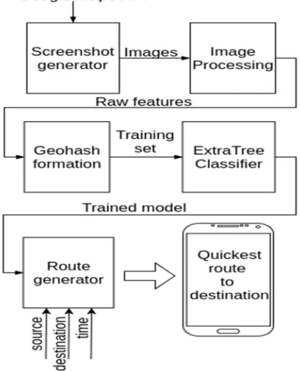
B. System Block Diagram

The entire process of system is shown in Fig. 1 as a Block Diagram. In the Block Diagram, there is one external interface, Google Maps API, and four modules, Screenshot generator, Image Processing, Geohash formation and ExtraTree Classifier training which works on server side. The results of these are stored on a database will be later used by client application. Route generator takes user input through the application and gives the best route using the trained models’ predictions. It takes source and destination addresses, records journey time and splits up alternative routes into segments for calculating predictions.

IV. IMPLEMENTATION DETAILS

The implementation of the system is composed of the following brief stages. In each stage alternative methodologies have been tried to choose the best one.

A. Pre-Processing

The first approach uses an unbiased approach for feature extraction. The pictures are filtered to remove all colours except those representing traffic. Next, sampling traffic begins. The features noted are the latitude, longitude obtained via shift of origin and scaling applied over pixel coordinates of the image. Other than these, time is noted as weekday, hour and minute obtained from creation time of the picture. The target value is one of the four classes, light traffic, medium traffic, heavy traffic and very heavy traffic, based on the corresponding colour shown on that coordinate. Without any further constraint, a huge amount of tuples might get extracted from a single picture. To avoid this situation, an upcoming latitude, longitude pair is considered only if there is no other existing sample in a 50m radius with the same target traffic. The minute’s value for each recorded tuple was floored down to the nearest 15th minute; this was necessary because the interval while capturing pictorial data was not exactly 15 minutes due to inherent system delay in triggering actions and fluctuating internet speeds required to load the map and traffic.

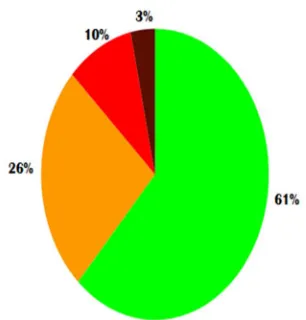
Fig. 2 Initial class distribution for first approach

The problem with the above technique is the highly imbalanced distribution of target traffic in the tuples extracted as seen in the Fig. 2. The major class covers roughly 60% of the data while the minor class covers only 3% of data. To tackle this, the minor class was discarded and two major classes were reduced to the size of the third class. This reduction was achieved by clustering the data of each of the two major classes into the same number of clusters as the size of the third class. Clustering was achieved by K-Means which is an unsupervised Machine Learning algorithm with an ability to cluster data into a known number of clusters. This process is time consuming as the total number of tuples are nearly 4,000,000 and two sets of 400,000 clusters are to be prepared from a set of 2,500,000 and 1,000,000 tuples. The resulting balanced classes are seen in Fig. 3.

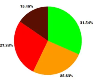
Fig. 4 Class distribution in second approach

In the second approach, the problem of imbalance is addressed at the ground stage itself by using a biased method to extract features from images. The entire Image Processing remains same, except that instead of sampling all target classes’ tuples at a fixed 50m, the major class is sampled at larger distances and minor class is sampled at very small distances apart. This gives us a dataset which is inherently less imbalanced and does not require clustering. All four target classes are usable and have good number of samples each as seen in Fig. 4. The imbalance issue doesn’t get completely solved here; during training in the further steps, the algorithm will be informed about weights of each class, dependent on ratio of the class in the dataset, which will be multiplied with the loss function to penalize the minor class more than the major one. This basically forces the algorithm to learn the minor class with more effort. There are approximately 4,000,000 tuples of data and with just 5 features in hand the model might end up underfitting. The latitude and longitude values form a very complex distribution which is tough to map by any math function; it will also not be scalable if new regions are used to train the algorithm. So, both these features are converted into a Geohash[12], which is a string of length 7. The Geohash algorithm assigns a hash value to all geolocations in the world and its precision is adjustable. The maximum precision available is +-11cm at a string length of 12. A string of length 7 gives precision of +-70m. The remaining features of weekday, hour and minutes are augmented using their squares as added features. So a total of 7 features are now available for the dataset. The traffic patterns change vastly with time and applying same parameters to the entire 24 hour cycle might not give best results. So periods of 3 hours are taken, generating 8 datasets over a period of 24 hours. Each dataset will be learnt by an individual model.

B. Machine Learning Algorithms

unconstrained environments, hence the tree depths were limited to 20 and the forest had 10 estimators (trees). There is one overfitting problem with Random Forest which exists due to the way its algorithm works. It uses a number of trees to learn sub samples of data which are decided from bootstrap tuples fixed at the beginning of the algorithm. To overcome this, Extra Trees algorithm[14] was tried which chooses samples from the entire training set for deciding the variables at the split as opposed to Random Forest which uses only the bootstrap samples. Other parameters of the algorithm were kept unchanged to avoid excessive deepening of the trees.

V. RESULTS

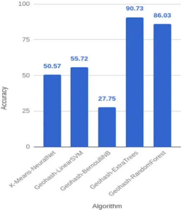
Having discussed the available alternatives, performance of each, post the training, was evaluated on an unseen test set. The five different algorithms used are henceforth referred as K-Means-NeuralNet, LinearSVM, BernoulliNB, Geohash-ExtraTrees and Geohash-RandomForest.

Fig. 5 comparing accuracies of alternative algorithms

Algorithm Green Orange Red Dark red

K-Means-NeuralNet -5.32 -18.73 24.05 0

Geohash-LinearSVM 20.18 -16.75 -4.52 1.09

Geohash-BernoulliNB -24.64 -19.94 -7.31 51.89

Geohash-ExtraTrees -0.21 -0.05 0.03 0.23

Geohash-RandomForest 1.43 -0.66 -0.55 -0.22

TABLE 1 Difference in expected and predicted distribution of output classes

The accuracies were calculated as the ratio of correct predictions with total predictions. In terms of accuracy, as seen in Fig. 5 the winner was Geohash-ExtraTrees closely followed by Geohash-RandomForest. Decision trees were found to well suit the problem and as expected, ExtraTree algorithm generalized better than RandomForest.

Fig. 6 Graphical view of difference in expected and predicted distribution of output classes

The results were collected from the confusion matrix prepared over the test set targets and predictions made over the test set features. Ratio of presence of each class was calculated as a percentage value. Looking at Fig. 6 generated from TABLE 1 it’s seen that again, ExtraTree and RandomForest algorithms have worked the best.

VI. CONCLUSION

Vehicular Traffic is an alarming issue that needs to be dealt with a solution quickly achievable. With the proposed supervised learning technique, which will be available to all via an android application, the problem can be mitigated in a dynamic manner. The solution is kept personal to cater to individual immediate needs of going from one place to another. It does not put a big toll on the devices’ performance as it works offline and avoids huge battery consumptions. It also helps to reduce the accident rate in the city. Currently, this solution lends data from the Google Maps API; alternative sources of data can be tested to improve the system. The implementation is targeting only Android OS; in future, other prominent mobile OS can be taken into consideration to expand the solution’s reach.

REFERENCES

[1] ThammasakThianniwet, SatidchokePhosaard and WasanPattara-Atikom, Classification of Road Traffic Congestion Levels from GPS Data using a Decision Tree Algorithm and Sliding Windows, Proceedings of the World Congress on Engineering 2009 Vol I WCE 2009, July 1 - 3, 2009.

[2] Advances in Human Machine Interaction (HMI - 2016), March 03-05, 2016.

[3] ArashJahangiri and Hesham A. Rakha, Applying Machine Learning Techniques to Transportation Mode Recognition Using Mobile Phone Sensor Data, IEEE, 2015

[4] CharlottVallon, ZiyaErcan, Ashwin Carvalho and Francesco Borrelli, A machine learning approach for personalized autonomous lane change initiation and control, IEEE Intelligent Vehicles Symposium (IV), 2017

[5] UrunDogan and Johann Edelbrunner and IoannisIossifidis, Autonomous Driving: A Comparison of Machine Learning Techniques by Means of the Prediction of Lane Change Behavior, Proceedings of the 2011 IEEE International Conference on Robotics and Biomimetics December 7-11, 2011.

[7] Jungme Park, Zhihang Chen, Leonidas Kiliaris, Ming L. Kuang, M. AbulMasrur, Anthony M. Phillips, and Yi Lu Murphey, Intelligent Vehicle Power Control Based on Machine Learning of Optimal Control Parameters and Prediction of Road Type and Traffic Congestion, IEEE TRANSACTIONS ON VEHICULAR TECHNOLOGY, VOL. 58, NO. 9, NOVEMBER 2009

[8] Anurag Sharma, Anurendra Kumar, K.V Sameer Raja, ShreeshLadha, Automatic License Plate Detection, IIT Kanpur, 2015-2016. [9] Justin Kestelyn, Real-time data visualization and machine learning for London traffic analysis, November 2016

[10] Simon Box and Ben Waterson, An automated signalized junction controller that learns strategies from a human expert, Draft of the paper in Engineering Applications of Artificial Intelligence, 2012

[11] Ryan Jay Herring, “Real-Time TracModeling and Estimation with Streaming Probe Data using Machine Learning”, Fall 2010 [12] Geohash.org. (2018). Geohash - geohash.org. [online] Available at: http://geohash.org/

[13] Duchi, John, EladHazan, and Yoram Singer. "Adaptive subgradient methods for online learning and stochastic optimization." Journal of Machine Learning Research 12.Jul (2011): 2121-2159.