Accepted
Article
This article has been accepted for publication and undergone full peer review but has not been through the copyediting, typesetting, pagination and proofreading process, which may lead to differences between this version and the Version of Record. Please cite this article as
DR. FREDERICK C DRAPER (Orcid ID : 0000-0001-7568-0838) MS. XIMENA TAGLE (Orcid ID : 0000-0003-4152-2051) Article type : Articles
Running head: Tree dominance and beta diversity
Dominant tree species drive beta diversity patterns in Western
Amazonia
Frederick C Draper 1,2*, Gregory P. Asner1, Eurídice N. Honorio Coronado3, Timothy R. Baker4, Roosevelt García-Villacorta5, Nigel C. A. Pitman6, Paul V.A. Fine7, Oliver L. Phillips4, Ricardo Zárate Gómez3, Carlos A. Amasifuén Guerra8, Manuel Flores Arévalo8, Rodolfo Vásquez Martínez9, Roel J.W Brienen4, Abel Monteagudo-Mendoza 9,10, Luis A. Torres Montenegro8, Elvis Valderrama Sandoval8, Katherine H. Roucoux11, Fredy R. Ramírez Arévalo12, Ítalo Mesones Acuy7, Jhon Del Aguila Pasquel 3,13, Ximena Tagle Casapia3, Gerardo Flores Llampazo14, Massiel Corrales Medina15, José Reyna Huaymacari8 and Christopher Baraloto2
Accepted
Article
1
Department of Global Ecology, Carnegie Institution for Science, Stanford, CA, USA
2
International Center for Tropical Botany, Florida International University, Miami, FL, USA
3
Instituto de Investigaciones de la Amazonía Peruana, Iquitos, Loreto, Perú
4
School of Geography, University of Leeds, Leeds, West Yorkshire, UK 5
Department of Ecology and Evolutionary Biology, Cornell University, Ithaca, NY, USA
6
Science and Education, The Field Museum, Chicago, IL, USA
7
Department of Integrative Biology, University of California, Berkeley, CA, USA
8
Facultad de Biología, Universidad Nacional de la Amazonía Peruana, Iquitos, Loreto, Perú
9
Jardín Botánico de Missouri, Oxapampa, Pasco, Perú
10
Universidad Nacional de San Antonio Abad del Cusco, Cusco, Perú
11
School of Geography and Sustainable Development, University of St Andrews, St Andrews, UK
12
Facultad de Ciencias Forestales, Universidad Nacional de la Amazonía Peruana, Iquitos, Loreto, Perú
13
School of Forest Resources and Environmental Science, Michigan Technological University, Houghton, MI, USA
14
Universidad Nacional Jorge Basadre Grohmann, Tacna, Perú
15
Universidad Nacional de San Agustín de Arequipa, Arequipa, Perú
Abstract
Accepted
Article
of them accounted for 50% of individuals. Using these 99 species it was possible to
reconstruct the overall features of regional beta diversity patterns, including the location and dispersion of habitat types in multivariate space, and distance-decay relationships. In fact, our analysis demonstrated that regional patterns of beta diversity were better maintained by the 99 dominant species than by the 1932 others, whether quantified using species abundance data or species presence/absence data. Our results reveal that dominant species are normally common only in a single forest type. Therefore, dominant species play a key role in
structuring Western Amazonian tree communities, which in turn has important implications, both practically for designing effective protected areas, and more generally for understanding the determinants of beta diversity patterns.
Key Words
Dominance, beta diversity, Western Amazonia, species turnover, tree species, common species, rare species, tropical forest communities, Loreto, habitat specificity
Introduction
A consistent pattern among all ecological communities is that few species are common and many are rare (Preston 1948, MacArthur 1957). Common species, by virtue of their high abundance, dominate key ecosystem functions such as primary productivity and biomass storage (Grime 1998), and therefore have a vital role in underpinning ecosystem services (Gaston and Fuller 2008, Gaston 2010). The hyper-diverse tree communities of Amazonia are no exception to this ‘few common and many rare’ rule, and a number of recent studies have emphasized that a small number (<5%) of tree species, termed ‘hyperdominants’ or
‘oligarchs’, account for the majority of individuals at large spatial scales (>100,000 km2
Accepted
Article
(Pitman et al 2001; Macía & Svenning 2005; Pitman et al 2013; ter Steege et al 2013; Pitman et al 2014). Amazon hyperdominants also dominate some ecosystem functions, for example,
~1 % of Amazonian tree species account for 50 % of stored biomass and woody productivity (Fauset et al. 2015). Despite our increased understanding of the functional importance of dominant species, little is known of their role in driving spatial patterns of community level turnover in species composition.
It is evident that in highly diverse ecosystems, such as Amazonian forests, it is rare species rather than common species that contribute the most to patterns of local and regional species richness (i.e. alpha and gamma diversity) (Hubbell 2013). The contribution that common species make to patterns of species turnover through space (i.e. beta diversity), on the other hand, is far less clear. In some other ecological systems, such as boreal tree communities and global avian populations, common species have a disproportionately strong influence on patterns of beta diversity (Nekola and White 1999, Gaston et al. 2007). However, the ecological literature presents a conflicting narrative regarding the potential importance of common species in determining patterns of beta diversity in tropical forests. On one hand, species that are common in one habitat type are more likely to be common in other habitat types than rare species (Pitman et al. 2001, 2014), suggesting that dominant species have broader habitat requirements than the average species, and will therefore decrease turnover among habitat types and will be a poor proxy of whole community patterns of beta diversity. On the other hand, patterns of species turnover in common species may be broadly
Accepted
Article
floristic similarity in tree communities is determined primarily by the most common species, with the removal of the most common 10% of species from the analysis having a much greater effect than the removal of the rarest 80% of species (Morlon et al. 2008).
In this paper we aim to investigate the role of dominant species in determining regional-scale patterns of tree beta diversity across a range of habitat types in Loreto, a 37 million ha region covering the Northern Peruvian Amazon basin. As beta diversity has been used to refer to a range of concepts and measurements in ecology (Tuomisto 2010, Anderson et al. 2011), we investigate three specific types of beta diversity pattern: 1) Floristic similarity among plots belonging to different habitat types; 2) Floristic similarity among plots within the same habitat type; and 3) The distance-decay of floristic similarity among plots within the same habitat type, which provides a measure of the turnover in species composition as a function of geographic distance.
Accepted
Article
H1a: Dominant species are poor predictors of beta diversity patterns among habitat types because they are common in several habitat types (i.e. habitat generalists).
H1b: Dominant species are good predictors of beta diversity patterns among habitat types when species abundance data are used but not when occurrence data are used, because although they occur in several habitat types they only achieve high abundance in a single habitat type.
H1c: Dominant species are always good predictors of beta diversity patterns among habitat types using both occurrence and abundance data because they occur most frequently in a single habitat type.
H2: Dominant species are poor predictors of distance-decay relationships within habitat types.
Accepted
Article
Methods
Forest inventories
Forest plot inventory data were taken from several contributing sources and, as a result, varied in plot size and sampling protocol used (Table 1). The compiled dataset consists of 207 forest plots covering the major forest habitat types in Loreto: terra firme forest, white-sand forest, seasonally-flooded forest, peatland pole forest and palm swamp forest (Figure 1). A summary of plot sources can be found in Table 1, and further details in Appendix S2. Most data were downloaded from the ForestPlots.net online database (Lopez-Gonzalez et al. 2011).
Standardizing datasets
As plot data came from several different sources and determinations were made by numerous different botanists, it was not possible to standardize our taxonomy across the entire dataset. As a result, individuals that could not be identified to species level were removed from the dataset and excluded from all subsequent analysis. We expect this removal of unidentified morphospecies to have little effect on our analysis of beta diversity. A similar plot-based study has shown strong correlations (R2 >0.98) between estimates of beta diversity
(ecological distances) including and excluding unidentified morphospecies (Pos et al. 2014). As plot size (and therefore the number of stems per plot) varied among our datasets we converted our abundance data into relative abundances (i.e. number of individuals per species/total individuals per plot).
Accepted
Article
rather than our environmentally biased dataset. To do this we estimated that the different habitat types account for the following proportions of forested land area in Loreto: Terra firme forest 60 %, seasonally-flooded forest 20 %, palm swamp 10%, white-sand forest 5 %,
peatland pole forest 5 %, based on the best maps of habitat types available in Loreto (Josse et al. 2007, Draper et al. 2014, Palacios et al. 2016, Asner et al. 2017). We then created a correction factor (actual proportion of habitat type area in plot dataset / predicted proportion of habitat type area). The abundance of each species in each plot was then multiplied by the corresponding correction factor. This corrected dataset provided an estimate of population size for each species within Loreto, and was used for all subsequent analysis.
Identifying dominant species
Dominant species were defined simply as the minimum number of species that together account for 50 % of all individual trees across the corrected dataset following the definition of ter Steege et al (2013). Species that were not identified as dominant have been labelled rare throughout the rest of the manuscript. We did not attempt to distinguish between the two dimensions of dominance, local abundance and regional frequency (Arellano et al. 2014), nor did we attempt to ensure a representative number of dominant species from each habitat type. Our definition was purposefully coarse, as we sought to frame our definition of dominance in the simplest terms.
Accepted
Article
excluding either 10 or 50% of plots at random from each habitat type in our dataset. We were then able to calculate the proportion of our list of dominant species that are found in these subsampled datasets.
Analysing patterns of beta diversity
In order to summarize patterns of beta diversity among plots both within and among habitat types, we used NMDS ordinations using the vegan package in R (Oksanen et al. 2013). NMDS ordinations were produced in two ways: Firstly, species abundance data were used to construct an ecological distance matrix using the Hellinger distance (Legendre and Legendre 2012), which was then used to construct the first NMDS ordination. This ordination provides a way of assessing how similar plots are to one another based on the abundance of tree species. Secondly, species presence/absence data was used to construct a different ecological distance matrix using the Jaccard index, this distance matrix then formed the basis for the second NMDS. This ordination provides a way of assessing how similar plots are to one another based on the occurrence of tree species. Both NMDS ordinations were optimized for two axes and run for 100 iterations or until a convergent solution was reached.
Quantifying dissimilarity within and among habitat types
To quantify floristic dissimilarity among habitat types we used the PERMANOVA method (Anderson 2001), which tests the significance of habitat types in determining plot locations in multivariate space. This method tests whether plots in the same habitat type are more
Accepted
Article
To quantify floristic dissimilarity within habitat types we used the multivariate dispersion method (Anderson 2006) to assess the dispersion of plots within each habitat type in
multivariate space. This method tests how floristically similar plots are to one another within each habitat type. The multivariate dispersion method was applied using the betadisper function in the R package vegan. Combined, these methods present a robust approach to identifying location vs dispersion effects in multivariate space (Anderson and Walsh 2013). We then compare how these statistics varied among the three datasets including: i) all species, ii) only dominant species and iii) only rare species.
To test whether the different minimum stem diameter cut-offs used across the plot dataset (ranging from 2 – 10 cm) had a significant impact on our analyses of beta-diversity, we repeated the distance-based ordination analyses using only those stems greater than 10 cm dbh. We found results from these repeat analyses to be remarkably consistent with the original analyses (Appendix S1: Fig S2, Table S2 and Table S3), and therefore these repeat analyses have not been discussed further.
Model based ordinations
Accepted
Article
Markov Chain Monte Carlo (MCMC) estimation in the R package boral (Hui 2016). Default model parameters were used apart from the fourth hyper parameter, which affects the
distribution of default priors, and was reduced from the default of 30 to 20 in order to reduce computational requirements and allow the model to run. Using the model output, posterior latent variable medians for each forest plot can then be plotted in an ordination, where the first two axes represents the two most important axes of floristic variation (Hui 2016).
Distance-decay analysis
To quantify the contribution of dominant species to the distance-decay of floristic similarity within forests types at a regional scale, we used binomial generalized linear models (GLMs). Geographic distance was the predictor variable and floristic similarity was the response variable, and a log link function was used following Millar et al. (2011). We conducted this analysis using both species abundance (standardised Hellinger distance) and
presence-absence data (standardised Jaccard index) for all species, only dominant species and only rare species. The average model fits along with the 95% confidence intervals surrounding these fits have been plotted in order to visualise the distance-decay relationships. This approach provides a measure of how species composition varies within forest types as a function of geographic distance.
Quantifying habitat specificity
Accepted
Article
habitat type for each species in the habitat type where that species is most abundant. We also ran this analysis once all species abundance values had been normalised to one, i.e. reduced the data set to presence/absence. We did this to ensure that our results were not dominated by single plots where common species have achieved exceptionally high abundance. Our second approach was to use indicator species analysis (Dufrêne and Legendre 1997), to assess which species are significant indicators of a particular habitat type. Indicator species analysis was conducted using the R package labdsv (Roberts 2013).
Quantifying the effect of under-sampling on patterns of beta diversity
To estimate the effect of under-sampling on patterns of beta diversity, we used a resampling procedure to purposefully under-sample dominant species. This procedure consisted of sampling a set number (5, 10, 15, or 20) individuals from each dominant species. These individuals were drawn at random from the Loreto-wide population of each dominant species. We then generated a Hellinger distance matrix and NMDS ordinations in the same way as was done with the original species pool.
Results
Identifying dominant species
From our dataset of 60,000 individual trees made up of 2031 species, we found that just 99 species (~5%; Appendix S1: Table S1) accounted for 50% of individual trees. Because these relatively few species collectively represent half of all trees in our dataset, we call them ‘dominants’, equivalent to the term ‘hyperdominant’ as used by others in the context of
Accepted
Article
In our simulation analysis, we found this list of 99 dominant species to be reasonably robust when 10% of the plot data was excluded, although the most abundant dominant species were more stable than the least abundant. For example, all of the 30 most abundant dominant species in our list were found in > 85% of the simulated datasets, while only 24 of the 30 least abundant dominant species occurred in the majority of simulated datasets. The list was far less robust in the simulations where 50% of the plot data were excluded. In these
simulations, all of the 30 most abundant dominant species were found in ~ 30% of the simulated datasets. Again, this became more pronounced with the less abundant dominant species; for example, only 15 of the 30 least abundant dominant species occurred in a majority of simulated datasets.
Floristic similarity among habitat types
The NMDS ordination figures constructed using all 2031 recorded species from the dataset show clear patterns, with plots clustering based on habitat type. This clustering by habitat type is significant (based on PERMANOVA tests) and consistent in ordinations constructed using both abundance and presence-absence data (Figure 2 panels A and B).
Accepted
Article
The ordination plots created using rare species (1932 species) also show broadly similar clustering patterns to ordinations that were constructed using all 2031 species or using only 99 dominant species (Figure 2; panels E and F). However, removing dominant species results in substantial overlap among palm-swamp and seasonally-flooded forest plots in ordinations constructed with both abundance and presence-absence data. This overlap is reflected in the PERMANOVA test which demonstrated that habitat types are least distinct when only rare species are included in the analysis (r2 =0.08, Table 2).
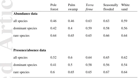
Floristic similarity within habitat types
Overall floristic similarity within habitat types increased when only dominant species were included and decreased when dominant species were excluded. The results from the
multivariate dispersion analysis suggest that average dispersion of plots within habitat types was consistently lowest when only dominant species were included, and dispersion was consistently highest in the dataset that included only rare species (Table 3).
Model-based ordinations
Accepted
Article
Distance-decay analysis
There are clear patterns in the distance-decay relationships within habitat types when all species are considered, both using abundance and presence/absence datasets (Figure 3 panels A and B). Peatland pole forests, palm swamp forests and seasonally-flooded forests all exhibit relatively steep declines in similarity with increasing distance between plots, whereas terra firme and white-sand forests are characterized by a much shallower distance-decay
pattern. The distance-decay models based on the 99 dominant species are similar to the models based on all 2031 species; however, there is an overall increase in similarity when rare species are excluded (Figure 3; panels C and D). This increase in similarity is especially evident in peatland pole forest and palm swamp habitat types, and when models are
constructed using presence/absence data. The distance-decay models based on the 1932 rare species were substantially different from models based on all species. Excluding dominant species led to lower overall similarity among plots within habitat types, as well as less variation in distance-decay rates among models of different habitat types (Figure 3; panels E and F). The gradient of all distance-decays models became more gradual as a result of excluding common species.
Habitat specificity analysis
Our analysis of habitat specificity demonstrated that most individuals of most species occurred in a single habitat type (Figure 5 panel B). Importantly, this was true of both
Accepted
Article
Once species abundances had been standardised to unity (i.e. converted to presence/absence), a similar pattern was found: Most species predominantly occur in a single habitat type, and again this was true for both dominant as well as for rare species (Figure 5 panel C). The mean proportion of per-species occurrences found in a single habitat type was 73% for dominant species and 78% for rare species. Again, the overlapping 95% confidence intervals on the boxplot indicate there is no significant difference between these two groups (Figure 5 panel C).
Finally, 317 species were identified as significant indicator species in our dataset (P ≤ 0.05). Of these significant indicators, 80 were dominant species (Appendix S1: Table S1), which is equivalent to 81% of dominant species. The remaining 237 indicator species represented just 12% of rare species.
The effect of under-sampling
Under-sampling dominant species had a strong effect on observed patterns of beta diversity (Figure 6). Previously observed patterns of among habitat type turnover within dominant species were still detectable (but less distinct) when 20 individuals were sampled per species. However, patterns became increasingly less pronounced when fewer individuals were
sampled. When five individuals were sampled per species, there was no evidence of clustering of plots into habitat types (Figure 6).
Discussion
Accepted
Article
that we observed are broadly consistent using either traditional distance-based multivariate approaches or a Bayesian model-based framework, suggesting that these results are not a product of using distance-based statistics. Furthermore, we found the same beta diversity patterns when analyses were conducted using either species abundance or species presence-absence data. This suggests that our results are not merely a product of dominant species controlling beta diversity patterns due to their exceptionally high abundance in individual plots, but rather that in general, dominant species are strongly associated with particular habitat types and localities.
How can so few species have such an important influence on regional scale patterns of beta diversity? Our analysis of habitat specificity demonstrates that most dominant species occur most frequently in a single habitat type, even though 88% of dominant species are found in more than one habitat type. Interestingly, dominant species in our dataset do not appear to be significantly less habitat specific than rare species, when considering either abundance or presence-absence of species. This pattern of similar habitat specificity persists despite the fact that we would expect rarer species to be more habitat specific by chance simply because they are likely to be under-sampled in our dataset. This finding therefore supports our third
hypothesis that dominant species are good predictors of beta diversity patterns among habitat types because they occur most frequently in a single habitat type. These results appear to contrast with previous findings in nearby forests, which have suggested that species that are dominant in one habitat type are more likely to occur in other habitat types (Pitman et al. 2001, 2014). However, only eight species from these previous studies were found to be ‘super oligarchs’, i.e. common across several habitat types, which is consistent with our
Accepted
Article
The results from the habitat specificity analysis suggest that dominant species are relatively specialized to a single habitat type, within which they may be functionally optimal. This within-habitat success may be explained by the growth-defense trade-off across edaphic gradients (Fine et al. 2006). This hypothesis states that the combination of impoverished soils and herbivory in low fertility habitats (e.g. white-sand forests) leads to higher investment in defense, while in high fertility habitat types (e.g. terra firme forest) species are more likely to invest more heavily in growth. Therefore, this mechanism would suggest that highly
successful dominant species are likely to have optimal traits for one habitat, which in turn leads to a trade-off against success in other habitat types. This habitat specific dominance may also allow dominant species to serve as source populations, supplementing neighbouring populations in sub-optimal habitat types, consistent with the concept of source-sink dynamics (Pulliam 1988). Such an interpretation would be consistent with the original oligarchy
hypothesis, which predicts that dominant species should only dominate in relatively homogeneous environmental settings (Pitman et al. 2013).
Our results also indicate that the reduced spatial patterns seen in rare species in our dataset results from under-sampling of these species. Our under-sampling simulations approach demonstrates that even when there is a strong underlying pattern, it can be masked if species are represented by fewer than 20 individuals (Figure 6). Given that approximately 75 % of species in our dataset are represented by fewer than 20 individuals, and half are represented by fewer than 6 individuals, under-sampling is likely masking patterns in rare species.
Indeed, when we attempted to isolate and examine patterns of beta diversity in the rarest 50% of species, we found no patterns in the data (Appendix S1: Figure S1). Therefore, it is
Accepted
Article
Therefore, it is reasonable to assume that it is not currently possible to describe the spatial patterns of abundance for most tropical forest tree species.
There is substantial overlap between our list of 99 dominant species and published lists of oligarchic species in Western Amazonia (Pitman et al. 2001, 2014) and hyperdominant species in the entire basin (ter Steege et al. 2013). Approximately 40% of species found on our list of Loreto dominants are also listed as oligarchs in upland terra firme or swamp forests (Appendix S1: Table S1) (Pitman et al. 2001, 2014). This overlap is somewhat
surprising as Pitman’s studies were conducted in more fertile regions closer to the Andes, did not consider pole forest or white sand forest habitat types, and used different criteria for defining dominance which incorporated both total species abundance and frequency in a given habitat type. There is even greater overlap between our list of dominant species in Loreto and Amazonian hyperdominants, with 47% of species in our Loreto list also occurring on the list of Amazonian hyperdominants (Appendix S1: Table S1). Again, this comes as some surprise as Loreto represents 6% of the area of Amazonia, and many Amazonian hyperdominants do not occur in Loreto. Moreover, our study includes peatland pole forest which is not included in the basin-wide analysis. Peatland pole forests are known to have a distinct composition, and several species (e.g. Tabebuia insignis and Cybianthus spicatus) would not be dominant if this forest type were excluded.
Practical implications
Accepted
Article
appear to be broadly representative of overall patterns of beta diversity. This is important because identifying these 99 dominant species is a more straight-forward task than a full tree species inventory, and taxonomic identifications are more likely to be valid for dominant species than for rarer species (Baker et al. 2017), although some dominant species may represent species complexes (Damasco et al. in press). As dominant species are functionally important and include species from most major clades, it may be more informative to focus on these common species than on a taxonomically restrictive list, when resources are limited, as has been suggested elsewhere (Higgins and Ruokolainen 2004, Ruokolainen et al. 2007). Rapid inventories of dominant species may highlight areas that are outliers in multivariate space and therefore may have a particularly distinctive flora. Examples from our dataset are the two plots OLL-03 and OLL-04, which are clear floristic outliers. These plots represent peatland pole forests that receive occasional inundation and have an extremely stunted canopy (~5m) heavily dominated by Cybianthus spicatus (Primulaceae) and the swamp specialist Tabebuia insignis var. monophylla (Bignoniaceae). To the best of our knowledge, these plots have provided unique floristic records of this habitat type in Amazonia, and therefore warrant further investigation.
Our results also have important implications for understanding the spatial ecology of tropical forests through remote sensing technologies. Recent advances using airborne imaging
spectroscopy have demonstrated that beta diversity can now be estimated at a landscape scale remotely (Féret and Asner 2014a, 2014b, Draper et al. 2018a). These approaches use
unsupervised machine learning to identify c. 30-50 “spectral species”, which are
Accepted
Article
multivariate space were sufficient to understand patterns of beta diversity at a regional scale (< 105 km2). Therefore, 50 multivariate features (e.g., spectral species) may be sufficient for understanding patterns of beta diversity at smaller landscape scales (> 100 km2) using imaging spectroscopy approaches. Furthermore, because dominant species make up a large fraction of the sunlit canopy, they play a key role in determining the identity of the species that constitute the forest functional classes (FFCs) that underpin national-scale functional beta-diversity (Asner et al. 2017). Therefore, our results suggest that dominant species are crucial to driving the turnover in large-scale functional composition in response to geologic substrate and elevation.
Limitations of this study
An important caveat of our approach is that in order to identify regionally dominant species, it is first necessary to assemble extensive regional floristic inventories of all species
Accepted
Article
Torres Montenegro et al. 2015). Yet M. carana is a very rare species in our dataset (8 individuals in total) and is therefore not included in our list of dominants.
Conclusions
In this study, we have highlighted the important role of dominant species in determining patterns of beta diversity within and among different habitat types in Western Amazonia. Dominant species are geographically widespread in Loreto, and while they may superficially appear to be widely occurring habitat generalists, our data set shows that they often
predominantly occur in single habitat types. Despite the widespread distribution of dominant species, it is possible to understand spatial patterns of beta diversity such as distance-decay relationships, using a heavily restricted dataset, consisting of only dominant species.
We have focused on the wealth of information to be gained by understanding a few dominant species, however, we caution that our findings do not diminish the value of rare species to understanding regional diversity patterns. Instead, this study reveals how little we know of the spatial ecology of most Amazonian tree species. Moreover, in this study, we have focused exclusively on the taxonomic dimension of beta diversity opposed to functional beta
Accepted
Article
into why some species achieve dominance, as well as revealing the underlying mechanisms that determine species distributions, which in turn govern patterns of beta diversity.
Acknowledgments
This study was supported through a joint project between the Carnegie Institution for Science and the International Center for Tropical Botany at Florida International University. GPA and FCD were supported by a grant from the John D. and Catherine T. MacArthur Foundation and the Leonardo DiCaprio Foundation. Plot installations, fieldwork and botanical
identification by the authors and colleagues has been supported by several grants including a NERC PhD studentship to FCD (NE/J50001X/1), an ‘Investissement d’avenir’ grant from the Agence Nationale de la Recherche (CEBA, ref. ANR-10- LABX-25-01), a Gordon and Betty Moore Foundation grant to RAINFOR, the EU’s Seventh Framework Programme (283080, ‘GEOCARBON’) and NERC Grants to OLP (Grants NER/A/S/2000/0053, NE/B503384/1,
Accepted
Article
Literature cited
Anderson, M. J. 2001. A new method for non‐ parametric multivariate analysis of variance. Austral ecology 26:32–46.
Anderson, M. J. 2006. Distance‐ based tests for homogeneity of multivariate dispersions. Biometrics 62:245–253.
Anderson, M. J., et al. 2011. Navigating the multiple meanings of β diversity: A roadmap for the practicing ecologist. Ecology Letters 14:19–28.
Anderson, M. J., and D. C. I. Walsh. 2013. PERMANOVA, ANOSIM, and the Mantel test in the face of heterogeneous dispersions: What null hypothesis are you testing? Ecological Monographs 83:557–574.
Arellano, G., L. Cayola, I. Loza, V. Torrez, and M. J. Macía. 2014. Commonness patterns and the size of the species pool along a tropical elevational gradient: insights using a new quantitative tool. Ecography 37:536–543.
Arellano, G., et al. 2016. Oligarchic patterns in tropical forests: role of the spatial extent, environmental heterogeneity and diversity. Journal of Biogeography 43:616–626.
Asner, G. P., et al. 2017. Airborne laser-guided imaging spectroscopy to map forest trait diversity and guide conservation. Science 355:385–389.
Baker, T. R., et al. 2017. Maximising Synergy among Tropical Plant Systematists, Ecologists, and Evolutionary Biologists. Trends in Ecology & Evolution 32:258–267.
Accepted
Article
Cardoso, P., P. A. V Borges, and J. A. Veech. 2009. Testing the performance of beta diversity measures based on incidence data: the robustness to undersampling. Diversity and Distributions 15:1081–1090.
Damasco, G., D. C. Daly, A. Vicentini and P.V.A. Fine. In Press. Reinstatement of Protium cordatum (Burseraceae) based on integrative taxonomy. Taxon.
Draper, F. C., et al. 2018a. Imaging spectroscopy predicts variable distance decay across contrasting Amazonian tree communities. Journal of Ecology.
Draper, F. C., et al. 2018b. Peatland forests are the least diverse forests documented in Amazonia, but contribute to high regional beta-diversity. Ecography 41:1–14.
Draper, F. C., et al. 2014. The distribution and amount of carbon in the largest peatland complex in Amazonia. Environmental Research Letters 9.
Dufrêne, M., and P. Legendre. 1997. Species assemblages and indicator species: the need for a flexible asymmetrical approach. Ecological monographs 67:345–366.
Fauset, S., et al. 2015. Hyperdominance in Amazonian forest carbon cycling. Nat Commun 6.
Féret, J.-B., and G. P. Asner. 2014a. Microtopographic controls on lowland Amazonian canopy diversity from imaging spectroscopy. Ecological Applications 24:1297–1310.
Féret, J.-B., and G. P. Asner. 2014b. Mapping tropical forest canopy diversity using high-fidelity imaging spectroscopy. Ecological Applications 24:1289–1296.
Fine, P. V. A., R. García-Villacorta, N. C. A. Pitman, I. Mesones, and S. W. Kembel. 2010. A Floristic Study of the White-Sand Forests of Peru. Annals of the Missouri Botanical Garden 97:283–305.
Accepted
Article
turnover across space and edaphic gradients in western Amazonian tree communities. Ecography 34:552–565.
Fine, P.V.A., Dávila, N., Foster, R., Mesones, I., and Vriensendorp, C. 2006. Vegetation and Flora. Pp 174-183 in Vriesendorp et al. (eds.) Perú: Matsés. Rapid Biological
Inventories Report 16. Chicago Illinois: The Field Museum.
Fine, P. V. A., et al. 2006. The growth-defense trade-off and habitat specialization by plants in Amazonian forests. Ecology 87:S150–S162.
García Villacorta, R., M. Ahuite Reátegui, and M. Olórtegui Zumaeta. 2003. Clasificación de bosques sobre arena blanca de la Zona Reservada Allpahuayo-Mishana. Folia
Amazonica 14:17–33.
Gaston, K. J. 2010. Valuing Common Species. Science 327:154–155.
Gaston, K. J., et al. 2007. Spatial turnover in the global avifauna. Proceedings of the Royal Society of London B: Biological Sciences 274.
Gaston, K. J., and R. A. Fuller. 2008. Commonness, population depletion and conservation biology. Trends in Ecology & Evolution 23:14–19.
Gentry, A. H. 1981. Distributional patterns and an additional species of thePassiflora vitifolia complex: Amazonian species diversity due to edaphically differentiated communities. Plant Systematics and Evolution 137:95–105.
Gentry, A. H. 1988. Tree species richness of upper Amazonian forests. Proceedings of the National Academy of Sciences 85:156–159.
Accepted
Article
Higgins, M. A., and K. Ruokolainen. 2004. Rapid Tropical Forest Inventory: a Comparison of Techniques Based on Inventory Data from Western Amazonia. Conservation Biology 18:799–811.
Honorio Coronado, E. N., J. E. Vega Arenas, and M. N. CorrallesMedina. 2015. Diversidad, estructura y carbono de los bosques aluviales del noreste Peruano. Folia Amazonica 24:55–70.
Hubbell, S. P. 2013. Tropical rain forest conservation and the twin challenges of diversity and rarity. Ecology and Evolution 3:3263–3274.
Hui, F. K. C. 2016. boral - Bayesian Ordination and Regression Analysis of Multivariate Abundance Data in r. Methods in Ecology and Evolution 7:744–750.
Hui, F. K. C., S. Taskinen, S. Pledger, S. D. Foster, and D. I. Warton. 2015. Model-based approaches to unconstrained ordination. Methods in Ecology and Evolution 6:399–411.
Josse, C., et al. 2007. Sistemas ecológicos de la cuenca amazónica de Perú y Bolivia. Clasificación y mapeo. NatureServe, Arlington.
Legendre, P., and L. Legendre. 2012. Chapter 7 - Ecological resemblance. Pages 265–335 in L. Pierre and L. Louis, editors. Developments in Environmental Modelling. Elsevier.
Leitão, R. P., et al. 2016. Rare species contribute disproportionately to the functional structure of species assemblages. Proceedings of the Royal Society of London B: Biological Sciences 283.
Lopez-Gonzalez, G., S. L. Lewis, M. Burkitt, and O. L. Phillips. 2011. ForestPlots.net: a web application and research tool to manage and analyse tropical forest plot data. Journal of Vegetation Science 22:610–613.
Accepted
Article
National Academy of Sciences 43:293–295.
Millar, R. B., M. J. Anderson, and N. Tolimieri. 2011. Much ado about nothings: using zero similarity points in distance-decay curves. Ecology: 92: 1717-1722.
Morlon, H., et al. 2008. A general framework for the distance-decay of similarity in ecological communities. Ecology letters 11:904–17.
Mouillot, D., et al. 2013. Rare Species Support Vulnerable Functions in High-Diversity Ecosystems. PLoS Biology 11:e1001569.
Nekola, J. C., and P. S. White. 1999. The distance decay of similarity in biogeography and ecology. Journal of Biogeography 26:867–878.
Oksanen, J., et al. 2013. Package ‘vegan.’ Community ecology package, version 2.
Palacios, J., et al. 2016. Mapeo de los bosques tipo varillal utilizando Imagenes de satelite rapideye en la provinica Maynas, Loreto, Peru. Folia Amazónica 25:25–36.
Pitman, N. C. A., et al. 2014. Distribution and abundance of tree species in swamp forests of Amazonian ecuador. Ecography 37:902–915.
Pitman, N. C. A., et al. 2008. Tree community change across 700 km of lowland Amazonian forest from the Andean foothills to Brazil. Biotropica 40:525–535.
Pitman, N. C. A., M. R. Silman, and J. W. Terborgh. 2013. Oligarchies in Amazonian tree communities: a ten-year review. Ecography 36:114–123.
Pitman, N. C. A., et al. 2001. Dominance and distribution of tree species in upper Amazonian terra firme forests. Ecology 82:2101–2117.
Accepted
Article
Preston, F. W. 1948. The Commonness, And Rarity, of Species. Ecology 29:254–283.
Pulliam, H. R. 1988. Sources, Sinks, and Population Regulation. The American Naturalist 132:652–661.
Räsänen, M. E., J. S. Salo, H. Jungnert, and L. R. Pittmantt. 1990. Evolution of the Western Amazon Lowland Relief : impact of Andean foreland dynamics. Terra Nova 2:320–332.
Roberts, D. W. 2013. Package ‘ labdsv .’ R package ver. 1.6–1:1–56.
Ruokolainen, K., H. Tuomisto, M. J. Macía, M. A. Higgins, and M. Yli-Halla. 2007. Are floristic and edaphic patterns in Amazonian rain forests congruent for trees,
pteridophytes and Melastomataceae? Journal of Tropical Ecology 23:13–25.
ter Steege, H., et al. 2013. Hyperdominance in the Amazonian tree flora. Science 342.
ter Steege, H., et al. 2003. A spatial model of tree α-diversity and tree density for the Amazon. Biodiversity & Conservation 12:2255–2277.
Stropp, J., H. Ter Steege, and Y. Malhi. 2009. Disentangling regional and local tree diversity in the Amazon. Ecography 32:46–54.
Torres Montenegro, L., T. et al. 2015. Vegetacion y flora. Pages 96–109 in N. Pitman, editor. Perú: Tapiche-Blanco. Rapid Biological and Social Inventories, report 27. The field museum, Chicago.
Tuomisto, H. 2010. A diversity of beta diversities: Straightening up a concept gone awry. Part 1. Defining beta diversity as a function of alpha and gamma diversity. Ecography 33:2–22.
Tuomisto, H., et al. 1995. Dissecting Amazonian biodiversity. Science 269:63–66.
Accepted
Article
comparison of fine-scale distribution patterns of four plant groups in an Amazonian rainforest. Ecography 23:349–359.
Warton, D. I., et al. 2015a. So Many Variables: Joint Modeling in Community Ecology. Trends in Ecology & Evolution 30:766–779.
Warton, D. I., S. D. Foster, G. De’ath, J. Stoklosa, and P. K. Dunstan. 2015b. Model-based thinking for community ecology. Plant Ecology 216:669–682.
Warton, D. I., S. T. Wright, and Y. Wang. 2012. Distance‐ based multivariate analyses confound location and dispersion effects. Methods in Ecology and Evolution 3:89–101.
Zárate Gómez, R., T. Mori Vargas, and L. Valles Pérez. 2013. Floristic composition, diversity and structure of white sand forest from the Allpahuayo-Mishana National Reserve, Loreto, Peru. Arnaldoa 19:237–247.
Accepted
[image:31.595.13.535.117.706.2]Article
Table 1. Summary of plot inventory data used in this analysis
Habitat type Terra firme forest Seasonally-flooded forest White-sand forest Palm swamp forest Peatland pole forest
No. plots 96 27 55 17 11
Plot size 0.1-1 0.5-1 0.025-1 0.1-0.5 0.5
Min. diameter
2.5 2.5 2 or 10 10[2] 10[2]
Total area (ha)
42.75 12.56 18.47 7.76 5.5
Total stems
33,815 7,006 20,742 4,818 9,427
Total species
1749 579 603 258 99
No. dominant species
87 71 54 43 24
No. indicator species
143 95 41 40 40
Reference Pitman et al. 2008; Honorio Coronado et al. 2009; Baldeck et al. 2016;
Baraloto et al. 2011; Phillips et al. 2003
Honorio Coronado et al. 2015; Baraloto et al. 2011
Fine et al. 2010; Baldeck et al. 2016; Baraloto et al. 2011; Zárate Gómez et al. 2013; Zárate Gómez et al. 2006; García Villacorta et al. 2003, Phillips et al. 2003
Draper et al. 2018
Accepted
Article
Table 2. PERMANOVA test results indicating the significance of habitat type in explaining
the location of plots in multivariate space based on either abundance data (Hellinger distance) or presence-absence data (Jaccard distance) for the entire dataset (all species), a subsampled data set using only dominant species and a subsampled dataset using only rare species.
F R2 P
Abundance data
all species 9.34 0.16 0.001
dominant species 14.43 0.22 0.001
rare species 4.5 0.08 0.001
Presence/absence data
all species 7.23 0.13 0.001
dominant species 15.46 0.23 0.001
Accepted
[image:33.595.25.509.179.451.2]Article
Table 3. Multivariate dispersal of plots within habitat types. Distances given are mean
Euclidean distances from plots to the median spatial location of each habitat type in NMDS multivariate space.
Mean distance from spatial median Pole
forest
Palm swamp
Terra firme
Seasonally flooded
White sand Abundance data
all species 0.46 0.46 0.63 0.63 0.59
dominant species 0.42 0.4 0.59 0.58 0.56
rare species 0.64 0.65 0.65 0.66 0.64
Presence/absence data
all species 0.52 0.6 0.64 0.65 0.62
dominant species 0.41 0.5 0.58 0.56 0.54
rare species 0.6 0.65 0.65 0.67 0.64
Figure 1. Map of field sites within the department of Loreto, Peru.
Figure 2. NMDS ordinations based on: data using all 2031 recorded species (panels A and
B); data using only 99 dominant species (panels C and D); and data using all 1932 rare species (panels E and F). Ordinations in the first column (panels A, C and E) were
Accepted
Article
Figure 3. Distance-decay curves among plots within five habitat types. Different rows
correspond to different datasets as follows: Panels A and B were made using data from all 2031 recorded species, panels C and D were made using only the 99 dominant species, panels E and F were made using all 1932 rare species. In the left column similarity is the inverse Hellinger distance derived from species abundance data, while in the right column similarity is the Jaccard index derived from species presence/ absence data. Lines represent mean GLM model fits, and shading represents 95% confidence intervals of model fits.
Figure 4. Latent variable model-based ordinations using posterior latent variable for each
plot if: all species are included in the model (panel A), only 99 dominant species are included in the model (panel B) and only 1932 rare species are included in the model (panel C).
Colours and shapes correspond to different habitat types: Purple triangles (terra firme forest); green diamonds (seasonally-flooded forest): yellow inverted-triangles (white-sand forests); red circles (peatland pole forests) and blue squares (palm swamp forest).
Figure 5. Distribution of habitat specificity for dominant and rare species. Habitat specificity
corresponds to the proportion of individuals of each species that are restricted to the habitat type where that species is most abundant (panel B). Panel C shows the same measure of habitat specificity when all abundances have been normalised to one (i.e. species
occurrences). Horizontal lines indicate median values, red points indicate mean values, boxes indicate the 25th and 75th percentiles, vertical lines indicate 1.5 x the inter-quartile range. Notches in boxes indicate approximate confidence intervals surrounding the median, therefore overlapping notches indicate no significant difference.
Figure 6. NMDS ordinations constructed with Hellinger distance matrices derived from