Munich Personal RePEc Archive
Synthetic data: an endogeneity
simulation
Carbajal De Nova, Carolina
Department of Economics, Autonomous Metropolitan University
13 February 2014
Synthetic data: an endogeneity simulation Working paper, February 13, 2014
Carolina Carbajal De Nova1
Department of Economics, Autonomous Metropolitan University [email protected]
Abstract
This paper uses synthetic data and different scenarios to test treatments for endogeneity problems under different parameter settings. The model uses initial conditions and provides the solution for a hypothetical equation system with an embedded endogeneity problem. The behavioral and statistical assumptions are underlined as they are used through this research. A methodology is proposed for constructing and computing simulation scenarios. The econometric modeling of the scenarios is developed accordingly with the feedback obtained from previous scenarios. The inputs for these scenarios are synthetic data, which are constructed using random number machines and/or Monte Carlo simulations. The outputs of the scenarios are the model estimators. The research results demonstrated that a treatment for endogeneity can be developed as the sample size increases.
Keywords: synthetic data, endogeneity problems, scenarios, Monte Carlo simulations.
1 Economics Professor (on leave). Av. San Rafael Atlixco, No. 186, Col. Vicentina, Del. Iztapalapa, Mexico
1. Introduction
This study develops a statistical application for providing an adequate treatment for endogeneity problems. The application is a hypothetical equation system that has an embedded endogeneity problem. This specification is a general form for the well-known endogeneity problem in economics. To characterize the evolution of the system of equations under different sample sizes and simulation scenarios, it is first necessary to create synthetic data as the equation system inputs. The synthetic data are constructed using Monte Carlo simulations based on the use of random number machines. In this respect, the author takes computational advantage of the already random machine modules installed in Matlab.
The main idea behind synthetic data is the creation of customized data and to feed a particular system of equations with them. The variation of key parameter values in the synthetic data and the variation of the sample size allow the implementation of a methodology to treat the endogeneity problem. Consequently, feasible tests are generated for demonstrating how the endogeneity problem decreases substantially under controlled conditions and without restrictions on data access. Thus, the proposed method adjusts the econometric modeling accordingly with the feedback obtained from previous scenarios. These different scenarios change when synthetic data and the system of equation parameter values take on different initial values. These changes respond to changes in assumptions. These scenarios represent behavioral experiments, which could have been very expensive had they been performed in real life. However, taking advantage of software developments and the increase of computational capacity in recent years, this research provides low-cost alternatives for performing these economic experiments or counterfactuals alongside their corresponding econometric tests and analyses. To the best of the author knowledge this endogeneity treatment approximation has not being discussed before in the literature.
This paper is organized as follows. Section 2 presents the model based on a system of equations, with an embedded endogeneity problem. Section 3 briefly describes the construction of synthetic data; implements the simulation scenarios and reports the corresponding results. The last section concludes.
2. Model
Consider the following equation in which income is a function of different demographics:
𝐼𝑛𝑐𝑜𝑚𝑒=𝛼!+𝛼
!𝑀𝑆+𝛼!𝐴𝑔𝑒+𝛼!𝐴𝑏𝑖𝑙𝑖𝑡𝑦+𝜖!
where 𝐼𝑛𝑐𝑜𝑚𝑒 stands for the returns of gaining a Master of Science degree; 𝑀𝑆 stands for
a Master of Science; 𝐴𝑔𝑒 stands for age; and 𝐴𝑏𝑖𝑙𝑖𝑡𝑦 stands for an unobservable variable that is linked with performance. The estimators are as follows: 𝛼! stands for the constant; 𝛼
! stands for
the 𝑀𝑆 estimator; 𝛼
! stands for 𝐴𝑔𝑒 estimator; 𝛼! stands for 𝐴𝑏𝑖𝑙𝑖𝑡𝑦 estimator; and 𝜖! stands for
the error term associated with this equation. This last term is assumed to be normal, independent and identically distributed, i.e., 𝜖
!~𝑁 0,𝜎!! .
𝐼𝑛𝑐𝑜𝑚𝑒=𝛼!+𝛼
!𝑀𝑆+𝛼!𝐴𝑔𝑒+𝜖!
where 𝜖
! stands for the error term associated with the 𝐼𝑛𝑐𝑜𝑚𝑒 variable, which contains
the unobservable 𝐴𝑏𝑖𝑙𝑖𝑡𝑦 variable.
Additionally, assume that 𝑀𝑆 has a Bernoulli distribution:
Pr 𝑀𝑆 =[𝜙 𝛾!+𝛾
!𝐴𝑏𝑖𝑙𝑖𝑡𝑦 ]
!"
+[1−𝜙(𝛾!+𝛾
!𝐴𝑏𝑖𝑙𝑖𝑡𝑦)]!!
!"
where Pr 𝑀𝑆 is the probability of observing the variable 𝑀𝑆; 𝐴𝑏𝑖𝑙𝑖𝑡𝑦 is the same variable
that appeared in the first equation; and 𝜙 stands for the standard normal cumulative distribution function (cdf).
Furthermore, assume that the next three assumptions hold:
Statistical assumptions
a) In deriving the method of moments estimator, the covariance expected value between regressors and the error term is zero, i.e., 𝐸 𝑋!𝜖 =0;
b) The variable 𝑀𝑆 is uncorrelated with the error term of equation (1). Then its
correlation is 𝜌!",!!=0.
Behavioral assumption
c) Negative quantities and prices only exhibit positive values.
Placing numbers to each of the equations above, the following system can be written:
𝐼𝑛𝑐𝑜𝑚𝑒=𝛼!+𝛼
!𝑀𝑆+𝛼!𝐴𝑔𝑒+𝛼!𝐴𝑏𝑖𝑙𝑖𝑡𝑦+𝜖!; (1)
𝐼𝑛𝑐𝑜𝑚𝑒=𝛼!+𝛼
!𝑀𝑆+𝛼!𝐴𝑔𝑒+𝜖!; (2)
𝑃𝑟 𝑀𝑆 =[𝜙 𝛾!+𝛾
!𝐴𝑏𝑖𝑙𝑖𝑡𝑦 ] !"
+[1−𝜙(𝛾!+𝛾
!𝐴𝑏𝑖𝑙𝑖𝑡𝑦)]!! !"
. (3)
A variable is said to be endogenous when there is a correlation between it and the error term.2 In the equation system above, the source of endogeneity seems to be related to the omitted
variable. This omitted variable could be 𝐴𝑏𝑖𝑙𝑖𝑡𝑦 if it is not observable. In fact, this should be true if the correct model is the one in equation (1), and the one that is feasible, given data availability, is the model depicted by equation (2). Since equation (3) establishes a relationship between
𝐴𝑏𝑖𝑙𝑖𝑡𝑦 and 𝑀𝑆, then the endogeneity problem could be revealed by means of the equation
system algebraic manipulation.
The first step in demonstrating the existence of the endogeneity problem in the above equation system is to show that equation (2) contains the omitted variable 𝐴𝑏𝑖𝑙𝑖𝑡𝑦. The second step consists of demonstrating that 𝑀𝑆 is correlated with the error term of equation (2): 𝜌!",! ≠ 0.
2 The use of a system of equations with a priory determination of exogenous and endogenous variables is
Consider that this hypothetical system has embedded an endogeneity problem. This problem is evidenced on equation (3). If equation (3) holds, then the correlation between 𝑀𝑆 and 𝐴𝑏𝑖𝑙𝑖𝑡𝑦 cannot be zero. Equation (3) links 𝐴𝑏𝑖𝑙𝑖𝑡𝑦 and 𝑀𝑆 through a non-linear relationship. For a
moment, assume that 𝐴𝑏𝑖𝑙𝑖𝑡𝑦 is observable and that equation (1) can be estimated. This means that the estimator 𝛼! can be computed. In this case, the specification of a correct statistical model
to commensurate income determinants is equation (1).
Now, consider that the variable 𝐴𝑏𝑖𝑙𝑖𝑡𝑦 cannot be observed. Equation (2) is then the only feasible model for estimation purposes. This implies that equation (2) replaces the econometric model of equation (1). However, if the correct model is the one set on equation (1), it implies that a measurement error associated with the omitted variable 𝐴𝑏𝑖𝑙𝑖𝑡𝑦 exists in equation (2). This last
idea can be represented as follows:
𝜖
!=𝛼!𝐴𝑏𝑖𝑙𝑖𝑡𝑦+𝜖!. (4)
Equation (4) shows that the omitted variable 𝐴𝑏𝑖𝑙𝑖𝑡𝑦 is absorbed into the error term of equation (2). Since the estimator 𝛼! is the one associated with 𝐴𝑏𝑖𝑙𝑖𝑡𝑦, it appears in equation (4).
Some partial weight of 𝜖 should also be present on 𝜖
!. For easiness, consider that 𝜖! is so small,
that some partial weight of it and itself have almost the same magnitude. In this case and for the sake of simplicity, equation (4) contains 𝜖
!.
The second step consists of showing that the correlation between 𝑀𝑆 and 𝜖
! is not zero if
equation (3) holds. Consider the following cross moment or conditional mean of 𝑀𝑆 given 𝜖:
𝐸 𝑀𝑆𝜖 =𝛽+ 𝑋!𝑋 !!𝑋!𝑍𝛿
Additionally, consider that the Gauss-Markov theorem holds for this case:
𝛽=(𝑋!𝑋)!!𝑋′𝑌
where 𝑌 stands for the variable 𝐼𝑛𝑐𝑜𝑚𝑒 and 𝑋 represents a set of independent variables.
Hence, the last equation can be rewritten as follows:
𝛽=(𝑋!𝑋)!!𝑋′(𝛼
!𝑀𝑆+𝛼!𝐴𝑔𝑒+𝛼!𝐴𝑏𝑖𝑙𝑖𝑡𝑦+𝜖!). (5)
where 𝑌 is written in terms of equation (1).
Suppose that 𝛼
!𝑀𝑆+𝛼!𝐴𝑔𝑒=𝑋𝛽;𝛼!𝐴𝑏𝑖𝑙𝑖𝑡𝑦=𝛿𝑍; Z stands for the instrumental variable
(IV); 𝛿 stands for the estimator of the IV; and
!=𝑈;𝑈 represents a generalized error term.
Making substitutions and distributing terms in this last expression, it can be written as follows:
𝛽=(𝑋!𝑋)!!𝑋′(𝑋𝛽+𝑍𝛿+𝑈)
𝛽=(𝑋!𝑋)!!𝑋′(𝑋𝛽)+(𝑋!𝑋)!!𝑋′𝑍𝛿+(𝑋!𝑋)!!𝑋′𝑈
𝛽=𝛽+(𝑋!𝑋)!!𝑋′𝑍𝛿+(𝑋!𝑋)!!𝑋′𝑈
𝐸 𝛽 𝑋 =𝛽+ 𝑋!𝑋 !!𝑋!𝑍𝛿
𝐸 𝛽𝑋 =𝛽+𝑏𝑖𝑎𝑠
The generalized estimator 𝛽 is biased if 𝑋!𝑍≠0 or 𝛿≠0.3 In this case, the bias is
represented by the term(𝑋!𝑋)!!𝑋′𝑍𝛿. This well-known result is the omitted variable formula.
In the last equation, 𝑏𝑖𝑎𝑠 is proportional to a weighted portion of 𝐴𝑏𝑖𝑙𝑖𝑡𝑦, which depends
on a non-linear association with 𝑀𝑆. This association is set on equation (3). Please note that 𝐵𝑖𝑎𝑠
does not depend on 𝐴𝑔𝑒, since this hypothetical equation system does not provide an equation where 𝐴𝑔𝑒 and 𝐴𝑏𝑖𝑙𝑖𝑡𝑦 are related.4
Another way to express 𝑏𝑖𝑎𝑠 is as follows:
𝐸 𝛽 𝑋 =𝛽+!"#!",!"#$#%& !"#!"
𝛼!. (6)
where 𝛼! is the 𝐴𝑏𝑖𝑙𝑖𝑡𝑦 estimator of equation (1).
From equation (4), it is known that 𝜖
!=𝛼!𝐴𝑏𝑖𝑙𝑖𝑡𝑦+𝜖!. Thus, 𝐴𝑏𝑖𝑙𝑖𝑡𝑦 can be expressed as
follows:
𝐴𝑏𝑖𝑙𝑖𝑡𝑦= 𝜖
!−𝜖!
𝛼!
Plugging the last expression for 𝐴𝑏𝑖𝑙𝑖𝑡𝑦 into equation (6) results in the following:
𝐸 𝛽 𝑋 =𝛽+
!"#!",!!!!!
!!
!"#!"
𝛼!. (6)’
If 𝛽 is 𝑏𝑖𝑎𝑠𝑒𝑑 as explained previously, then it should follow that
!"#!",!!!!!
!! !"#!"
𝛼!≠0 and
thus 𝑐𝑜𝑣 𝑀𝑆,!!!!!
!!
≠0.
The correlation coefficient for the 𝑀𝑆 and 𝐴𝑏𝑖 𝑖𝑡𝑦 variables is as follows:
𝜌!",!"#$#%&=𝑐𝑜𝑟𝑟 𝑀𝑆, 𝐴𝑏𝑖𝑙𝑖𝑡𝑦 =!"#!(!",!"#$#%&)
!"!!"#$#%& , or
𝜌
!",!!!!!!
!
=𝑐𝑜𝑟𝑟 𝑀𝑆, 𝜖
!−𝜖! 𝛼! =
𝑐𝑜𝑣(𝑀𝑆,𝜖!𝛼−𝜖! ! )
𝜎!"𝜎!!!!! !!
3 For an example containing endogeneity bias, see Hayashi (2000) [7] (p. 187).
since 𝑐𝑜𝑣 𝑀𝑆,!!!!! !!
≠0, and 𝜖
!~𝑁(0,𝜎!!) it follows that 𝜌!",!!!!! !!
≠0. Thus, there is
indeed a correlation between 𝑀𝑆 and 𝜖
!. With these two steps, the endogeneity problem
embedded in the hypothetical equation system has been made evident, since it matched the definition of an endogenous variable: an endogenous variable exists when there is a correlation between it and the error term. This applies specifically to 𝑀𝑆 in equation (2).
Once the endogeneity problem has been made evident in the equation system, what follows is the specification for synthetic data construction and simulation scenarios. These procedures are presented in the next section. The construction of synthetic data can be done in different ways. One is by means of Monte Carlo simulations, which are widely used. It uses a recursive algorithm and a fix population. The seed fixes the population to a given size. Therefore, its seed limits Monte Carlo sample sizes. The use of random machines, which are modules preinstalled on Matlab, allows samples to be drawn from an infinite population. These samples have asymptotic properties that are absent in samples derived from Monte Carlo simulations.5
The author opts for this last method, since it results in samples with asymptotic properties. In the next section, the synthetic data and construction of scenarios are explained.
3. Results
Consider the next four stages for describing synthetic data construction and scenario estimations:
1. Take initial parameter values for the variables that composed equations (1); (2) and (3): 𝛼!,𝛼
!,𝛼!,𝛼!,𝛾!,𝛾!,𝜎!!;
2. With the help of the random number generators, which are modules preinstalled on Matlab, generate 20 observations for each variable in this research equation system;
3. Proceed to estimate the income equation with different sample sizes, i.e., 50 and 100 observations. Compare these equation estimators in terms of percentage deviations from initial parameter values. Register the results properly in the corresponding tables;
4. Changing initial parameters values reproduces alternative scenarios. Let steps 2 and 3 adjust automatically to these new values and take note.
It is important to underline that the variables created in steps one and two represent synthetic data. They are generated with random number machines, and every time the run button is hit in the Matlab software, the algorithm is updated. This allows omitting the step of taking draws from the determined size of one population, as when the Monte Carlo method is used. This is the case because this procedure restricts the draws that could be taken given a certain population size. Regardless of whether Monte Carlo or the random machines method is used, both allow for the creation of synthetic data.
5 “Since the variables were generated with random number [generators], every time the code is run, the
variables get updated. This allows the analyst to omit an additional step of taking draws from the population in the Monte Carlo simulation. So, the population from which the samples are being taken is
Equation (2) was solved using 𝑀𝑆 synthetic data. This is important because it allows it to
have a determined distribution and asymptotic properties. That is, the population moments are shared by the synthetic data samples. The variable 𝑀𝑆 is key to estimating the system of
equations and to showing an endogeneity problem treatment.
For instance, assume that 𝐴𝑏𝑖𝑙𝑖𝑡𝑦 is not available. Thus, equation (2) nests the variable
𝐴𝑏𝑖𝑙𝑖𝑡𝑦 in its error term as described in equation (4). Furthermore, assume that 𝐴𝑏𝑖𝑙𝑖𝑡𝑦 is available
and denote it with the name 𝐴𝑏𝑖𝑙𝑖𝑡𝑦𝑏𝑖𝑠 to distinguish it from the case when it is not observable. The Pr(𝑀𝑆) on equation (3) can then be computed given that the variable 𝐴𝑏𝑖𝑙𝑖𝑡𝑦𝑏𝑖𝑠 is used as an
input. Using these two types of variables, 𝐴𝑏𝑖𝑙𝑖𝑡𝑦 and 𝐴𝑏𝑖𝑙𝑖𝑡𝑦𝑏𝑖𝑠, the differences of having an endogenous problem without and with treatment will become obvious in the next section. The treatment implements the use of IV. Instrumental variables are a common method in economics to correct endogeneity problems.
3.1. First scenario n=20 observations case
Follow steps 1-3 from the previous section. Set the number of repetitions to 20, for each of the variables on equations one to three. Initial parameter values are assigned as follows:
𝛼!=10;
𝛼 !=20;
𝛼 !=30.
After running a regression for equation (2) using the method of ordinary least squares, the following estimators are obtained:
𝛼!=41.7398; 𝛼
!=19.9312; 𝛼
!=30.1700.
The estimator for𝛼
! is closed to its assigned value. The difference between them is
(30.17-30)/30*100=0.56% (overestimation). Something similar occurs with 𝛼
!, where the difference
between the true value and its estimator is close to (19.9312-20)/20*100=-0.344% (underestimation). Regarding the coefficient estimate for 𝛼!, it is very far from its true value.
The following 95% confidence intervals are obtained after running the corresponding regressions:
For 𝛼!=41.7398, [13.3659 70.1137], with a true value of 𝛼!=10;
for 𝛼
!=19.9312, [19.4721 20.3904], with a true value of 𝛼!=20;
for 𝛼
!=30.1700, [29.4188 30.9213], with a true value of 𝛼!=30.
As we can see from the information given above, the confidence interval contained the truth-value. One exception is represented by 𝛼!. For instance, 𝛼
!=20 is contained in the
confidence interval [19.4721 20.3904]. Likewise, 𝛼
The coefficient estimate for 𝑀𝑆 (𝛼
!) is close to the lower bound of its 95% confidence
interval. The coefficient estimate for 𝐴𝑔𝑒 (𝛼
!) is near to the upper bound of its 95% confidence
interval. The coefficient for the constant (𝛼!) represents merely the average of the observations, so
it is around the middle of its 95% confidence interval.
n= 50 observations case, results
𝛼!=75.8929; 𝛼
!=19.8502; 𝛼
!=30.0290.
Remember that the following values for the above parameters are assigned as follows:
𝛼!=10; 𝛼
!=20; 𝛼
!=30.
The estimate for𝛼
! is closed to its assigned value. The difference between them is
(30.0290-30)/30*100=0.09% (overestimation). Something similar occurs with 𝛼
!, where the
difference between the estimate and its true value is close to (19.8502-20)/20*100=-0.749% (underestimation). Regarding the coefficient estimate for 𝛼!, it is very far from its true value.
n= 100 observations case, results
𝛼!=129.2581;
𝛼
!=19.9555;
𝛼
!=29.9135.
Remember that the following values for the above parameters are assigned as follows:
𝛼!=10; 𝛼
!=20; 𝛼
!=30.
The estimate for𝛼
! is close to its assigned value. The difference between them is
(29.9135-30)/30*100=-0.288% (underestimation). Something similar occurs with 𝛼
!, where the difference
between the estimate and its true value is close to (19.9555-20)/20*100=-0.222% (underestimation). Regarding the coefficient estimate for 𝛼!, it is very far from its true value.
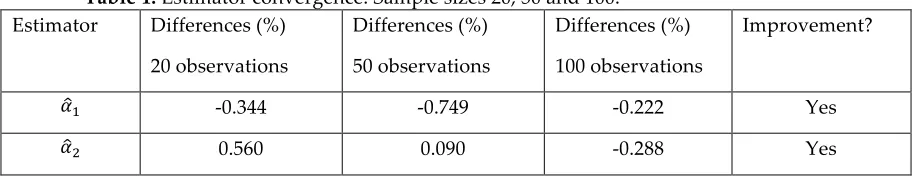
The differences of the estimates with 100 observations and the previous estimates with 20 and 50 observations, are compared in Table 1. This comparison aims to verify whether there is an improvement in the estimator convergence with its initial value, given an increase in the sample size.6
6 According to Kuh et al. (1985) [11], the process of varying the number of observations affects the
Table 1. Estimator convergence. Sample sizes 20, 50 and 100. Estimator Differences (%)
20 observations
Differences (%)
50 observations
Differences (%)
100 observations
Improvement?
𝛼
! -0.344 -0.749 -0.222 Yes
𝛼
! 0.560 0.090 -0.288 Yes
From Table 1, the differences measured in percentage terms have decreased as the number of observations increased in the sample. For instance, the difference between the estimator and its true value for 𝛼
! is -0.344% with 20 observations, and it decreases to -0.749%
with 50 observations; thus, this percentage decreases. It decreases even more with 100 observations, i.e., -0.222% (in absolute terms); thus, the percentage decreases. A similar improvement is seen in 𝛼
! because it passes from 0.56% with 20 observations to 0.09% with 50
observations and -0.288 with 100 observations; thus, the percentage decreases.
From Table 1, it can be confirmed empirically that as the number of observations increases, the coefficient estimates become closer and closer to their true values. This is simply a confirmation of the Law of Large Numbers, the Central Limit Theorem and the Asymptotic Distribution of the OLS estimators.7 The intuition is that as the number of observations increases
to infinity, the estimators will converge with their initial value. Remember that this research equation system has embedded an endogeneity problem. Convergence is possibly achieved, because the increase in sample size diminishes the estimator bias, and the aforementioned asymptotic properties hold. If this intuition is true, then this research results are aligned with those of Alvarez and Arellano (1988) [1] and Anderson and Hsiao (1981) [2].8
3.2. Second scenario
In the scenario above, the variable 𝐴𝑏𝑖𝑙𝑖𝑡𝑦 was unobservable. This assumption has now changed and 𝐴𝑏𝑖𝑙𝑖𝑡𝑦 is observed. This observable variable is called 𝐴𝑏𝑖𝑙𝑖𝑡𝑦𝑏𝑖𝑠. Equation (3) can be rewritten in terms of this observable variable.
Pr 𝑀𝑆 =[𝜙 𝛾!+𝛾!𝐴𝑏𝑖𝑙𝑖𝑡𝑦𝑏𝑖𝑠 ] !"
+[1−𝜙(𝛾!+𝛾
!𝐴𝑏𝑖𝑙𝑖𝑡𝑦𝑏𝑖𝑠)]!! !"
. (3)’
The initial parameter values for this scenario are:
𝛼!=10;
𝛼
!=50;
7 For a clear demonstration of the Central Limit Theorem, see Hogg et al. (2013) [9] (p. 307). More
information is available on Hamilton (1994) [6] regarding the Law of Large Numbers and Asymptotic Distributions.
8 When Alvarez and Arellano derive the asymptotic properties of different kind of estimators (GMM, LIML
𝛼 !=30;
𝛾!=40; 𝛾!=50;
𝜎 !!=1.
where 𝜎
!! represents the variance of the error term; 𝛾! and 𝛾! represent the estimators of
equation (3).
In this scenario, equation (2) includes equation (3)’. This implies that 𝑀𝑆 has been
computed in a previous stage and is later entered as input in equation (2).
n= 20 observations case
The estimators for equation (2) are:
𝛼!=126.2643; 𝛼
!= 20.2350;
𝛼
!= 30.0320.
The associated 95% confidence intervals are:
For 𝛼!=126.2643, [117.7658 134.7627], with a true value of 𝛼!=10;
for 𝛼
!=20.2350, [20.0225 20.4475], with a true value of 𝛼!=50;
for 𝛼
!=30.0320, [29.7946 30.2694], with a true value of 𝛼!=30.
From the information above, the confidence intervals do not contain the true initial value for 𝛼! and 𝛼
!. That is, 𝛼!=10 is not inside the range of the following interval [117.7658 134.7627]; 𝛼
!=50 is not contained in [20.0225 20.4475]. Reversing this behavior trend, we see that 𝛼!=30 is
contained in [29.4188 30.9213]. This behavior is likely observed, because now equation (2) nests equation (3)’.
n= 50 observations case
Once the sample size is increased from 20 to 50 observations, the following estimators are computed:
𝛼!=128.6414;
𝛼
!= 20.0608; 𝛼
!= 29.9382.
n= 100 observations case
𝛼!=23.1880; 𝛼
!=49.9987; 𝛼
!=30.1105.
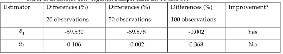
Table 2. Estimator convergence. Sample sizes 20, 50 and 100. Estimator Differences (%)
20 observations Differences (%) 50 observations Differences (%) 100 observations Improvement? 𝛼
! -59.530 -59.878 -0.002 Yes
𝛼
! 0.106 -0.002 0.368 No
From Table 2, it can be observed that the differences measured in percentage terms have decreased as the number of observations increased from 20 to 50. For instance, the difference between the estimator 𝛼
! and its true value is 59.530% with 20 observations, and it decreases to
-59.878% with 50 observations; it decreases even more with 100 observations, i.e., -0.002 (in absolute terms). The difference for the estimator 𝛼
! and its true value decreases when the sample
size increases from 20 to 50 observations, with values of 0.106 and -0.002, when the number of observations increases from 50 to 100, there is no improvement in its difference.
In general, Table 2 shows empirically that as the number of observations increases, 𝛼
!
estimators become closer and closer to its true value. This is simply a confirmation of the Law of Large Numbers, the Central Limit Theorem and the Asymptotic Distribution of the OLS estimators, as explained previously. In the case of 𝛼
!, convergency is not achieved, since the
endogeneity problem is now included in the estimation of equation (2).
3.3. Third scenario
Proceed to find a Generalized Method of Moments (GMM) for equation (2). Consider
𝐸(𝑍𝜖
!)=0 moment condition. When this moment condition holds, it replaces the standard
orthogonal condition and the derivation of a GMM estimator can be found, for the income equation:
Pr 𝑀𝑆 =[𝜙 𝛾!+𝛾
!𝐴𝑏𝑖𝑙𝑖𝑡𝑦𝑏𝑖𝑠 ]
!"
+[1−𝜙(𝛾!+𝛾
!𝐴𝑏𝑖𝑙𝑖𝑡𝑦𝑏𝑖𝑠)]!! !"
. (3)’
Taking the log in both sides of equation (3)’ produces the following expression:9
𝑙𝑛Pr 𝑀𝑆 =𝑙𝑛[𝜙 𝛾!+𝛾
!𝐴𝑏𝑖𝑙𝑖𝑡𝑦𝑏𝑖𝑠 ] !"
+𝑙𝑛[1−𝜙(𝛾!+𝛾
!𝐴𝑏𝑖𝑙𝑖𝑡𝑦𝑏𝑖𝑠)]!! !"
𝑙𝑛Pr 𝑀𝑆 =ln{[𝜙 𝛾!+𝛾
!𝐴𝑏𝑖𝑙𝑖𝑡𝑦𝑏𝑖𝑠 ] !"
1−𝜙 𝛾!+𝛾
!𝐴𝑏𝑖𝑙𝑖𝑡𝑦𝑏𝑖𝑠 !! !"
}
Applying the exponential to the last line yields the following:
Pr 𝑀𝑆 =[𝜙 𝛾!+𝛾
!𝐴𝑏𝑖𝑙𝑖𝑡𝑦𝑏𝑖𝑠 ] !"
1−𝜙 𝛾!+𝛾!𝐴𝑏𝑖𝑙𝑖𝑡𝑦𝑏𝑖𝑠 !! !"
. (7)
This last equation has a similar form as the Bernoulli probability density function (pdf):10
𝑝 𝑥 =𝑝![1−𝑝]!!!,𝑥=0,1. (8)
9 With this operation the corresponding equation is linearized. The corresponding estimators from the
equation with and without log should be equivalent, because they differ only in scale. Kantz and Schereiber (2003) [10] (p. 109) provide further insight regarding this equivalence.
When 𝑥 takes on values of 0 and 1, an indicator function is produced. The population
moments for a Bernoulli pdf are as follows:
𝜇=𝑝
𝜎!=𝑝[1−𝑝]
Equalizing equations (7) and (8) yields the following:
𝑝=𝜙(𝛾!+𝛾!𝐴𝑏𝑖𝑙𝑖𝑡𝑦𝑏𝑖𝑠)
Thus, the moments of the population are as follows:
𝜇=𝜙(𝛾!+𝛾
!𝐴𝑏𝑖𝑙𝑖𝑡𝑦𝑏𝑖𝑠)
𝜎!=𝜙(𝛾!+𝛾
!𝐴𝑏𝑖𝑙𝑖𝑡𝑦𝑏𝑖𝑠)[1−𝜙(𝛾!+𝛾!𝐴𝑏𝑖𝑙𝑖𝑡𝑦𝑏𝑖𝑠]
The sample moments for equation (8) are as follows:
1
𝑛 𝑥!
!
!!! =
𝑥
1
𝑛 𝑥!
!− 1
𝑛 𝑥! !
!!!
!
!
!!! =
𝑠!
where 𝑥 is the sample mean and 𝑠! is the sample variance.
To link the theory to the data, take the population moments (theoretical moments) and sample moments (empirical moments) and equalized them. Solve the following system of two equations:
𝑝=𝑥
𝑝 1−𝑝 =𝑠!
Solving this system yields the following:
𝑝=𝑥
𝑝 1−𝑝 =𝑥−𝑥!
Thus, a synthetic data can be constructed for 𝐴𝑏𝑖𝑙𝑖𝑡𝑦𝑏𝑖𝑠, considering that the theoretical and empirical moments values of 𝜇=𝑝=𝑥, and 𝜎!=𝑝 1−𝑝 =𝑥−𝑥! are equal. In this way,
the reliability of inference based on its statistical adequacy is secured. Additionally, these results are backed by the analytical model, which gauges the same functional relationships, information and optima among the relevant variables.11
Once constructed, 𝐴𝑏𝑖𝑙𝑖𝑡𝑦𝑏𝑖𝑠 generates a standard normal cdf from the random uniform variable 𝐴𝑏𝑖𝑙𝑖𝑡𝑦𝑏𝑖𝑠 with the values of 𝜇=0 and σ!=1. This computation will produce the
variable 𝑝=𝜙(𝛾!+𝛾!𝐴𝑏𝑖𝑙𝑖𝑡𝑦𝑏𝑖𝑠). This procedure assures that the previous computation is
correct.
Equation (7) can represent a probit model. Its log likelihood function is as follows:
𝑙𝑛𝑃𝑟 𝑀𝑆 =𝑀𝑆𝑙𝑛 𝜙 𝛾!+𝛾
!𝐴𝑏𝑖𝑙𝑖𝑡𝑦𝑏𝑖𝑠 + 1−𝑀𝑆 ln[1−𝜙 𝛾!+𝛾!𝐴𝑏𝑖𝑙𝑖𝑡𝑦𝑏𝑖𝑠 ]
The maximum likelihood estimator for the variable 𝑀𝑆𝑙𝑛 𝜙 𝛾!+𝛾
!𝐴𝑏𝑖𝑙𝑖𝑡𝑦𝑏𝑖𝑠 is 2.887,
with a standard error of 0.927. These figures for 1−𝑀𝑆 ln 1−𝜙 𝛾!+𝛾!𝐴𝑏𝑖𝑙𝑖𝑡𝑦𝑏𝑖𝑠 are -1.875
and 0.916, respectively.
Thus, plugging the above estimators values into equation (7) a value for 𝑀𝑆 can be
obtained. Table 3 reports the results after estimating the corresponding equation system for different sample sizes.
n= 20 observations case
The initial parameter values for this scenario are as follows:
𝛼!=10; 𝛼
!=20;
𝛼
!=30.
After running a regression for equation (2) using the method of ordinary least squares, the following estimators are obtained:
𝛼!=32.9122; 𝛼
!=0.0000;
𝛼
!=27.6321.
n= 50 observations case
𝛼!=109.3834;
𝛼
!=0.0000; 𝛼
!=29.2389.
n= 100 observations
𝛼!=81.0565;
𝛼
!=−0.0000;
𝛼
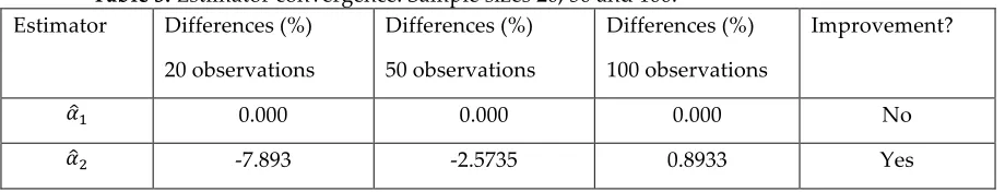
Table 3. Estimator convergence. Sample sizes 20, 50 and 100. Estimator Differences (%)
20 observations
Differences (%)
50 observations
Differences (%)
100 observations
Improvement?
𝛼
! 0.000 0.000 0.000 No
𝛼
! -7.893 -2.5735 0.8933 Yes
From the results reported in Table 3, it can be noted that the estimate coefficient for 𝛼 ! is
0 for 20; 50 and 100 observations. The GMM method provides unbiased estimators since its differences with the initial parameter value are zero. It seems that the hypothetical equation system is correctly identified with a Bernoulli pdf. Thus, 𝛼
! results imply that 𝐴𝑏𝑖𝑙𝑖𝑡𝑦𝑏𝑖𝑠 has an
impact close to zero on income determination. For its part, 𝛼
! displays convergence with its
initial value as the sample size increases.
3.4. Four scenario
This scenario includes the use of IV to correct the endogeneity problem of the second scenario. The variable Z is referred as the instrument or IV.
To determine whether 𝐴𝑏𝑖𝑙𝑖𝑡𝑦𝑏𝑖𝑠 could be used as IV, it is necessary to compute the correlation coefficient between 𝐴𝑏𝑖𝑙𝑖𝑡𝑦𝑏𝑖𝑠 and 𝜖
!. Note that in the model section, it was found that
𝜌
!",!!!!! !!
≠0. In this scenario, the correlation needed is 𝜌!"#$#%&"#'
,!!. It can be computed with the
aid of synthetic data: 𝜌!"#$#%&"#',!!=−0.0050. This value is close to zero. It is decided that this
empirical correlation coefficient value is almost zero and that 𝐴𝑏𝑖𝑙𝑖𝑡𝑦𝑏𝑖𝑠 and 𝜖
! are not correlated.
The theoretical justification for the use of instrumental variables can be found in Greene (2012). Remember that 𝐴𝑏𝑖𝑙𝑖𝑡𝑦𝑏𝑖𝑠 is observable to the econometrician.
The IV assumptions are as follows:
• Exogeneity. They are uncorrelated with the error term 𝐸(𝑍′𝜖
!)=0, where 𝑍′
indicates IV transpose;
• Relevance. They are correlated with the independent variables.
The asymptotic properties of the IV estimator indicate in general, that if 𝑍 has a finite variance, then the remaining regression equation components also have a finite variance:
𝑝𝑙𝑖𝑚 𝑍
!𝜖 !
𝑛 =𝑝𝑙𝑖𝑚
𝑍!𝑌
𝑛 −𝑝𝑙𝑖𝑚
𝑍!𝑋𝛽
𝑛 =0
Rearranging,
𝑝𝑙𝑖𝑚 𝑍
!𝑌
𝑛 = 𝑝𝑙𝑖𝑚
𝑍!𝑋
𝑛 𝛽+𝑝𝑙𝑖𝑚
𝑍!𝜖
! 𝑛
If 𝑝𝑙𝑖𝑚 !!!!
! =
𝑝𝑙𝑖𝑚 𝑍
!𝑌
𝑛 = 𝑝𝑙𝑖𝑚
𝑍!𝑋
𝑛 𝛽+0
𝑝𝑙𝑖𝑚 𝑍
!𝑌
𝑛 = 𝑝𝑙𝑖𝑚
𝑍!𝑋
𝑛 𝛽
If 𝑍 has the same number of variables as 𝑋, then the rank of 𝑍!𝑋 is k. This implies that 𝑍!𝑋
is a square matrix and its inverse exists:
𝛽= 𝑝𝑙𝑖𝑚 𝑍
!𝑋
𝑛 !!
𝑝𝑙𝑖𝑚 𝑍 !𝑌
𝑛
This last expression in closed-form leads to the IV estimator:
𝑏!"=(𝑍!𝑋)!!𝑍′𝑌
In this case, consider the following values for 𝜎
!!; 𝛾! and 𝛼!:
𝛼
!=50; 𝛾!=50; 𝜎
!!=2.
The corresponding estimators and their differences with respect to the initial parameters values are reported in Table 4.
n= 20 observations
𝛼!=17.4690; 𝛼
!=0.0000; 𝛼
!=31.4482.
n= 50 observations
𝛼!=109.3834; 𝛼
!=0.0000;
𝛼
!=29.2389.
n= 100 observations
𝛼!=137.6044;
𝛼
!=−0.0000; 𝛼
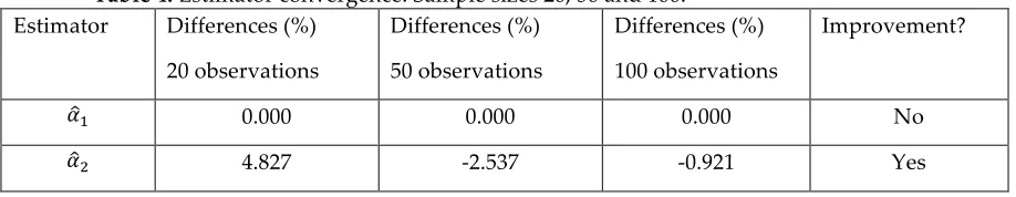
Table 4. Estimator convergence. Sample sizes 20, 50 and 100. Estimator Differences (%)
20 observations
Differences (%)
50 observations
Differences (%)
100 observations
Improvement?
𝛼
! 0.000 0.000 0.000 No
𝛼
! 4.827 -2.537 -0.921 Yes
After changing the parameters values for 𝜎
!!; 𝛾! and 𝛼!, it is found that the variable 𝑀𝑆
continues to exhibit a virtually null impact over the determination of income as in Table 3. These results are already explained by Swamy et al. (2017) [13] uniqueness definition. This implies that
MS was only statistically significant for the econometric model when it incorporates the omitted variable 𝐴𝑏𝑖𝑙𝑖𝑡𝑦. Once an endogeneity treatment based on the IV 𝐴𝑏𝑖𝑙𝑖𝑡𝑦𝑏𝑖𝑠 is implemented, the
variable MS stops being a relevant factor in the determination of income.
4. Conclusions
By increasing the sample size, the income estimators begin converging with the assigned initial parameter values. Perhaps these estimators become consistent, implying efficiency and a decreasing bias as an asymptotic result. Once the endogeneity problem embedded in a hypothetical equation system is controlled by the observable IV 𝐴𝑏𝑖𝑙𝑖𝑡𝑦𝑏𝑖𝑠, it is found that 𝑀𝑆 has
virtually a nil impact in the determination of income. This result suggests that 𝑀𝑆 has nothing to
do with the determination of income and that the statistical inference from scenarios 3.1. and 3.2. is incorrect, since they have the endogeneity problem without treatment. Scenario 3.3. GMM statistical adequacy secures identification and reliability of inference. Scenario 3.4. treats the endogeneity problem by means of IV and its results are the same under different initial parameter values with those of scenario 3.3. The recommendation derived from the use of synthetic data and simulation scenarios is to find an exogenous determinant of income to avoid incorrect statistical inference induced by the endogeneity problem. In case that exogenous determinants of income or adequate IV are not available, a feasible treatment for endogeneity by means of synthetic data consist in increasing the sample size. This recommendation has its empirical validation on the counterfactuals implemented in each simulation scenario.
Acknowledgments: I am indebted with Cornell University and Autonomous Metropolitan University for their facilities to finish this study.
Conflicts of Interest: The author declares no conflict of interest.
References
1. Alvarez, J.; Arellano, M. The Time Series and Cross-Section Asymptotics of Dynamic Panel
Data Estimators; Working Paper 9808; Center for Monetary and Financial Studies (CEMFI):
Madrid, Spain, 1998.
2. Anderson, T.W.; Hsiao, C. Estimation of Dynamic Models with Error Components.
Journal of the American Statistical Association. 1981, 76, 598-606.
4. Casella, G.; Berger, R.L. Statistical Inference, Duxbury Press: Pacific Grove, CA, USA, 1990. 5. Greene, W.H. Econometric Analysis, 7th ed.; Pearson, Prentice Hall: Upper Saddle River, NJ, USA, 2012.
6. Hamilton, J.D. Time Series Analysis, Princeton University Press: Princeton, NJ, USA, 1994. 7. Hayashi, F. Econometrics, Princeton University Press: Princeton, NJ, USA, 2000.
8. Hart, P.E.; Mills, G.; Whitaker, J.K. Econometric Analysis for National Economic Planning, Butterworths: London, UK, 1964.
9. Hogg, R.V.; McKean J.W.; Craig, A.T. Introduction to Mathematical Statistics, Pearson, Prentice Hall: Upper Saddle River, NJ, USA, 2013.
10. Kantz, H.; Schereiber, T. Nonlinear Time Series Analysis, Cambridge University Press: Cambridge, UK, 2003.
11. Kuh, E.; Neese, J.W.; Hollinger, P. Structural Sensitivity in Econometric Models, John Wiley & Sons: New York, NY, USA, 1985.
12. Spanos, A. Foundational Issues in Statistical Modeling: Statistical Model Specification and Validation. Rationality, Markets and Morals. 2011, 2, 146-178.
13. Swamy, P.A.V.B.; Mehta, J.S; Chang, I.L. Endogeneity, Time-Varying Coefficients, and Incorrect vs. Correct Ways of Specifying the Error Terms of Econometric Models. Econometrics