some organic chemicals. In fact, some thermal de-compositions have been shown to be autocatalytic. It therefore may be well to considerSash distillation of the crude product prior to subjecting it to fractional distillation to remove trace non-volatiles and/or non-volatiles which would accelerate decomposition or lead to excessively high pot temperatures. In some cases one might consider the addition of a stabilizing agent to the pot to retard decomposition.
Closing Remarks
With all of the above having been stated, fractional distillation, particularly at reduced pressure, can be viewed as an opportunity to see physical chemistry at work. When selecting a system one hopes will result in satisfactory partition of components it will be
helpful to consider properties other than the boiling point. For example, if a mixture of intermolecularly bound substances is to be separated by distillation, their partition is likely to be more difRcult than the differentials between their boiling points would indi-cate. On the other hand, a mixture of alkanes may well be more easily separable than comparison of their boiling points would otherwise indicate. In any case practice is necessary, both conducting distilla-tions and selecting systems for distillation. Once ex-perience has been gained it is satisfying to be able to rationalize the results of a fractionation in terms of physico-chemical principles. One positive note: since distillation does not result in loss of product, in the worst case one can recombine all the fractions and redistill using different conditions and, if necessary, a different system.
Modelling and Simulation
J. R. Haas, UOP LLC, Des Plaines, Illinois, USA
Copyright^ 2000 Academic Press
Introduction
Rigorous computer modelling of all types of frac-tionation columns has become a necessary part of the development and design process. There are numerous software products available to do these calculations. An understanding of the basic mathematics used in these programmes is helpful to select, use and troubleshoot a column model. Explained here are the basic equations, numerical and solution methods commonly used.
Stage and Column Models
A rigorous method describes a column as a group of equations and is the mathematical engine to solve and satisfy these equations to calculate the operating con-ditions of the column.
Column design and performance calculations pres-ent the column at steady state, that is, what pres-enters the column matches what leaves it (material and energy balances), i.e.:
(molar feedSow rates)
" (molar productSow rates) (mass feedSow rates)
" (mass productSow rates)
(moles of any component in the feeds)
" (moles of the component in the products) Feed enthalpy#Heat added
"Product enthalpy#Heat removed
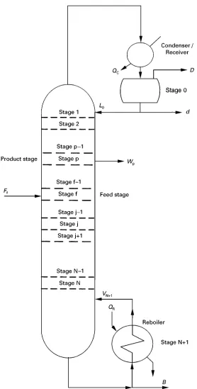
Figure 1 shows a complex column with one feed and one side product. The top stage of the column is a partial condenser, with a vapour product,D, and a liquid product,d. The reSux is the liquid,L0, and the reSux ratio isL0/(D#d). The bottoms product,
B, leaves stage N#1, the reboiler. The stages are numbered from the top, with the condenser as stage 0, the top tray in the column, stage 1, the bottom tray, stage N, and the reboiler, as stage N#1.
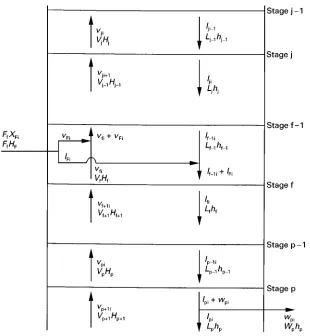
An ideal or equilibrium stage is where vapour and liquid entering and leaving the stage are perfectly mixed and there are no inhibitions to material trans-fer between the phases. The material and energySows in and out of a simple stage, with no feeds or side products, is stagejdepicted in Figure 2, andi repres-ents the component number. Componrepres-ents are num-bered from 1 to the last,C.
The enthalpy terms,Hjandhj, are molar enthalpies of the vapour and liquid leaving the stage, respective-ly. These molar enthalpies are multiplied by the total Sow rates,VjandLj, leaving the stage to give the total energy leaving the stage in each phase.
Figure 1 Overall column model with external variables.
with the liquid entering the feed stage while feed vapour mixes with vapour leaving the stage (though special consideration is made for the vapour feed at the bottom of absorber/stripper columns). The distri-bution is found by an adiabaticSash of the feed at the
Figure 2 Model of stage variables.
Similar models are drawn for the bottom and top stages of any column, plus other equipment such as product withdrawal stages (stage p of Figure 2), pump-around returns and draws, and inter-reboilers and inter-condensers. Since a reSux, reboiler vapour, feeds, or returns are often subcooled, superheated, or very different in composition from the material on the stage, the assumption of an equilibrium stage rapidly becomes invalid.
Equations of Distillation Modelling
The basic equations below fully describe a distillation column. These equations deRne the overall column total material balances, energy balances, and product compositions. Internal to the column, they describe equilibrium conditions, internal (stage-to-stage) com-ponent and total material balances, and internal energy balances. The independent variables of a col-umn are the product rates and compositions, internal vapour and liquid rates and compositions, and stage temperatures. Equilibrium constants, also called
Kvalues, and mixture enthalpies are dependent
vari-ables. Each stage is assumed to be at equilibrium (a theoretical stage), though an efRciency can be applied in the equations.
The equations wereRrst referred to as the MESH equations by Wang and Henke (1966). The MESH acronym stands for:
Material orSow rate balance equations, both com-ponent and total.
Equilibrium equations including the bubble and dew point equations.
Summation or Stoichiometric equations or com-position constraints.
Heat or enthalpy or energy balance equations. The MESH variables are referred to as state variables. These are:
E Stage temperatures,Tj
E Internal total vapour and liquid rates,VjandLj E Stage compositions,yjiandxji, or instead,
The equilibrium equation is:
yji"Kjixji or vji/Vj"Kjilji/Lj
The equilibrium constant or K-value, Kji, can be a complex function itself, dependent on the composi-tions,xjiandyji
Kji"Kji(Tj,Pj,xji,yji)
The dependence ofKji onxji andyjioften appears in the MESH equations. The component rates can also be expressed in the terms of each other, giving:
vji"lji(KjiVj/Lj)"ljiSji and
lji"vji(Lj/KjiVj)"vjiAji
KjiVj/Lj is termed the stripping factor, Sji, while
Lj/KjiVjis termed the absorption factor,Aji.
The summation equation or composition con-straints simply states that the sum of the mole frac-tions on each stage is equal to unity. For the liquid phase:
C
i"1
xji!1"0 or C
i"1
lji/Lj!1"0 or C
i"1
yji/Kji!1"0
and for the vapour phase: C
i"1
yji!1"0 or C
i"1
vji/Vj!1"0 or C
i"1
Kjixji!1"0
For a simple column (single feed, no side products), the overall component balance equation is:
fi!di!bi"0
The component balance for the simple stage (no feed or side product),j, of Figure 2, is:
vji#1#lji\1!vji!lji"0
The component balance for feed stage, f, of Figure 2 will add the liquid portion of the feed,lFi, while the vapour portion,vFi, is added to the component bal-ance for stage f!1. For the product stage, p, the
material withdrawn,wpi, is subtracted from the com-ponent material balance. By convention, material leaving a tray has a negative value and material enter-ing a tray has a positive value.
The total material balances are organized in the same manner as the component balances. The total material balance for the simple stage of Figure 2 is:
Vj#1#Lj\1!Vj!Lj"0
The same convention applies to feed and product trays where the totalSow rate of a feed,Ff, is positive and the product,Wp, is negative.
The equilibrium equation and the composition constraint are combined to get the bubble point equa-tion:
1 C i"1lji*
C
i"1
Kjilji!1"0 and the dew point equation:
1 C i"1vji*
C
i"1
vji
Kji
!1"0
These, or some variation, are important in some methods toRnd the stage temperature, especially for more narrow boiling mixtures.
The energy balance equations are required in any rigorous method. In narrow-boiling mixtures, they inSuence the internal totalSow rates. In wide-boiling mixtures and in columns where there are great heat effects (e.g. oil reRnery fractionators) they also strongly inSuence stage temperatures. The overall energy balance for a column with one feed and side product is:
FHF!DHD!BhB!WHW#QR!QC"0 The enthalpy terms,Handh, are per mole of mixture. Note that the enthalpies of the top and side products are written so that a vapour or liquid enthalpy can be substituted, depending on the phase of the product. The energy balance for the simple stage, j, of Figure 2 is:
vj#1Hj#1#Lj\1hj\1!VjHj!Ljhj"0 The enthalpies (energy per mole) for each phase are functions of temperature, pressure and com-position:
Hj"Hj(Tj,Pj,yji)
For feed stages, side product stages, and stages with inter-condensers or inter-reboilers, additional terms are included in the energy balance equations. The energy balance for the reboiler is:
LNhN!VN#1HN#1!BhN#1#QR"0 and for a partial condenser with both vapour and liquid products:
V1H1!L0h0!dh0!DH0!QC"0 Subcooling is accounted for inh0(the enthalpy of the reSux,L0, and the liquid distillate,d).
Most computer simulations work with ideal stages but to characterize a stage for the deviation from ideality or equilibrium, stage efRciencies are often used in some software. Commonly, a Murphree vapour efRciency is used for each component, given as:
EMVji"
yji!yji\1
yHji!yji\1
whereyHji is what the vapour composition would be if the vapour were in equilibrium with the actual liquid on the stage andyjiandyji\1are actual vapour com-positions. If the absorption factor is used, the vapour efRciency can be expressed in terms of variables al-ready presented:
EMVji"
vji!vji#1(Vj/Vj#1) (KjiVj/Lj)lji!vji#1(Vj/Vj#1)
A vaporization efRciency,Eji, based on the Murphree efRciency is deRned as:
Eji"EMVji#(1!EMVji)
yji#1
Kjixji
This can be used in the MESH equations to account for stage nonideality. This vaporization efRciency is applied to the equilibrium constant,Kji, and appears as the productEjiKji. The vaporization efRciency does solve a computational problem in placing an efR cien-cy in the MESH equations. A major disadvantage of the vaporization efRciency is that it does vary with composition. Near the top of a high purity column, as
yji#1 and xji approach unity, Eji also approaches unity, and so a vaporization efRciency does not truly reSect stage nonidealities.
Another efRciency method is the bypass method where some of the vapourSow of a component enter-ing the stage is sent to the next stage to account for its
inefRciency in separation. The bypass method cannot be used on trays that have material leaving or enter-ing from outside the column such as a feed tray, product draw tray, pump-around return or draw tray, or side-stripper return or draw tray. The bypass method will cause one of these trays to be out of mass balance. Some of the trays adjacent to these trays are also affected by these actions. In some columns, this eliminates a large number of trays and makes results difRcult to apply.
Caution then should be used in any choice of efR -ciency. More often, it is usually best to perform the rigorous calculation using ideal stages and then apply an overall column efRciency based on sound engineer-ing judgement and experience to account for stage nonideality, and calculate the number of actual trays or packing height.
Rigorous Computational Methods
Classi\cation of the Methods
The rigorous methods can be divided into four basic classes. These are:
E The bubble point methods (BP) E The sum-rates methods (SR) E The 2NNewton methods
E The global Newton or simultaneous correction (SC) methods.
The BP methods get their name because the stage temperatures are found by directly solving the bubble point equation. The BP methods generally work best for narrow-boiling, ideal or nearly ideal systems; where composition has a greater effect on temper-ature than the latent heat of vaporization.
The sum-rates (SR) method is suitable for model-ling absorbers and strippers with extremely wide-boiling systems, especially those with non-conden-sables. In these columns, temperatures are the domi-nant variables and are found by a solution of the stage energy balances. Compositions do not have as great an inSuence in calculating the temperatures as do heat effects or latent heats of vaporization.
The Rrst three classes are referred to as equation tearing or decoupling methods because the MESH equations are divided and grouped or partitioned and paired with MESH variables to be solved in a series of steps. The SC methods attempt to solve all of the MESH equations and variables together. Additional classes are:
E Inside-out methods E Relaxation methods
E Homotopy}continuation methods E Nonequilibrium models.
The relaxation, inside-out and homotopy} con-tinuation methods are extensions of whole or part of theRrst four methods in order to expand the range of columns, and to solve difRcult systems or columns. The nonequilibrium models are rate-based or trans-port phenomena-based methods that do away alto-gether with the ideal stage concept and eliminate any use of efRciencies. They are best suited for columns where a theoretical stage is difRcult to deRne and efRciencies are difRcult to predict or apply by any means.
Numerical Methods^The Newton^Raphson Technique
The MESH equations form a large system of inter-related, nonlinear, algebraic equations. The mathe-matical method used to solve all or part of these equations as a group is the Newton}Raphson method. An understanding of the numerical method is needed to understand the performance of all column methods. Detailed discussion of the Newton} Raphson method and its variations can be found in Holland’s (1981) text.
The Newton}Raphson is an approximation tech-nique. It assumes in the derivatives that the MESH equations are linear over short distances and the slopes will point towards the answers. The MESH equations can be far from linear and the predictions can take the next trial well off the curves, and move away from the solution. In some rigorous methods based on Newton}Raphson, a poor set of starting values can cause the calculation never to approach a solution. Also, the calculation can oscillate, with values swinging to either side of the solution. The independent variables calculated in a trial need to move the column to a solution. The software should include means to prevent or detect these problems and improve stability, e.g. by damping or limiting the change to the next set of variables. A Newton} Raph-son method will normally take even steps toward the solution.
Global Newton Methods
One group of methods that is very popular is the global Newton methods, also called the simultaneous correction (SC) methods. A common one is that of Naphtali and Sandholm (1971), but there are numer-ous applications in the literature and global Newton methods have been extended to include additional equations and variables for solving three-phase and reactive distillation columns.
In the global Newton methods, all of the equations are solved together in a Newton}Raphson technique. The methods vary in their choice of variables and MESH equations for the Newton}Raphson calcu-lation but none of the MESH equations are solved in any separate step. In the BP, SR and 2N Newton methods, the component balances and compositions lag the other MESH calculations (sinceKvalues and enthalpies are generated using the compositions from the previous trial) and compositions of each compon-ent are calculated independcompon-ently of the others MESH variables. These are major disadvantages with highly nonideal systems, whereKvalues (especially activity coefRcientsji) and enthalpies are highly composition dependent and where the composition of one com-ponent cannot be readily decoupled from those of others. The global Newton method includes the com-ponent balances among the Newton}Raphson inde-pendent functions and compositions join other MESH variables as independent variables.
The global Newton methods are the most sensitive of the rigorous methods to the quality of the initial values and often require initial values near the answer. This, and applying the methods to a full range of column equipment and speciRcations, is their greatest problem. Variations on global Newton methods are used in the inside-out, relaxation, homotopy and nonequilibrium methods, where their power and reliability is extended.
Inside-out Methods
The inside-out algorithm has become one of the most popular methods because of its robustness and its ability to be applied to the solution of a wide variety of columns. The inside-out concept was developed by Boston (1980). Russell (1983) presented an inside-out method that works well for many reRnery frac-tionators. The inside-out methods are now the methods of choice for mainstream column simulation and have displaced other methods.
an outer loop with the K values and enthalpies updated whenever the MESH variables change. The inside-out concept reverses this by using the complex
Kvalue and enthalpy correlations to generate para-meters for simpleKvalue and enthalpy models. These parameters are unique for each stage and become the variables for the outside loop. The inside loop consists of the MESH equations and is a variation on other methods. In every step through the outside loop, the simple models are updated using MESH variables from the inside loop. This sets up the next pass through the inside loop. Since theKvalues and enthalpies are simple, the inside loop works well for a wide range of mixtures and is little affected by the nonideality of mixtures or the quality of the initial values.
The outer loopKvalue model is based on a simple composition-independentKmethod:
lnKbj"Aj#Bj(1/Tj!1/TH)
whereTHis a reference temperature for theKvalue correlation. Outer loop variables,AjandBj, are gen-erated for each stage from a referenceKbjRefof a com-posite component:
lnKbjRef" C
i"1
wilnKji(actual)
where the wi are weight factors. The temperatures and compositions used to get the Kji(actual) are the latest from the inside loop. Simple relative volatil-ities are among the outside loop variables, and are used in the Kb method to calculate the temper-atures and wheneverKvalues are needed in the inside loop:
ji"Kji(actual)/KbjRef
These simple relative volatilities change little over the range of temperatures that is seen on a given stage and greatly simplify temperature and composition calculations in the inside loop. For nonideal mixtures, an activity coefRcient for each component accounts for composition effects in the inside loop. This activ-ity coefRcient has a simple model, similar to the
Kbmodel:
lnHji"aji#bjixji
where the new outer loop variables, aji and bji, for each component are determined from the actual ac-tivity coefRcient model at the current stage temper-ature and stage composition.
The simple K values used in the inside loop are easily determined from:
Kji(simple)"KbjjiHji
Simple models for the enthalpy of a phase are also used to reduce effects such as that caused by compo-nents moving past their critical conditions. Thus, the outside loop calculation consists of updating the terms of the simple K value, activity and enthalpy models which are updated after each inside loop solution using the latest temperatures and composi-tions from the inside loop.
The inside loop consists of the actual calculation of the MESH variables using the simple K value and enthalpy models. Boston initially used an inside loop solution method similar to a bubble point method and from that it may appear that the Boston method is most appropriate for narrow-boiling mixtures. However, the forcing style of the method also allows it to work well for wide-boiling mixtures. The Boston method works well for tall, high purity (superfrac-tionator) type columns, but has been extended to absorbers, to three-phase distillation, and to reactive distillation by using other arrangements of the MESH equations.
The Boston method includes a middle loop to allow for column speciRcations and constraints. The ar-rangement of equations in the inner loop, where the solution of the MESH variables occur, may allow for only a few control or speciRed variables, such asRxed reSux ratio and product rates. The middle loop ad-justs the control variables to meet the speciRcations. The middle loop can be built as an optimization method with process speciRcation equations and eco-nomic objectives and constraints.
Russell’s (1983) method differs from Boston’s in the inside loop by a solution method of the MESH equations that includes speciRcations for product quality, stage temperatures, internalSow rates, etc., without the use of a middle loop to solve these. Here, for each heat exchanger in the column, plus each additional side product, an additional speciRcation and operating variable is added to the problem. Rus-sell’s method has been found to work well for reRnery fractionators with side strippers and other similar columns.
Relaxation Methods
state distillation equations. These unsteady-state equations are modiRcations to the MESH equa-tions to include changes in the MESH variables with respect to time. This mimics the physical start-up of the column, but the objective is not to follow the dynamic operation but to seek the steady-state solution.
Homotopy^Continuation Methods
Homotopy or continuation methods are applied to difRcult-to-solve columns, and are a simple means of forcing a solution. The MESH equations can be difR -cult to solve, due either to the nature of the column (many feeds or side products, side strippers, near minimum reSux, etc.) or to the nonidealities of the
Kvalues or enthalpies. For three-phase systems, azeo-tropic systems or systems of columns with two or more feed/recycle stream combinations, there may be more than one calculated solution. The method must be forced to reach the desired solution. Homotopy methods begin with a known solution of the column and from there follow a path to the desired solution. The known solution can be at different conditions or with much simplerKvalue and enthalpy methods and stepped changes are made from there, solving the column equations at each step, until theRnal solution is reached.
Nonequilibrium or Rate-based Methods
Stage efRciency prediction and scale-up from ideal or equilibrium stages to the actual design can be difRcult and unreliable for many columns. For highly nonideal, polar and reactive systems, such as amine absorbers and strippers, prediction and use of ef-Rciencies is particularly difRcult. In such mixtures, mass transfer and not equilibrium often limits the separation.
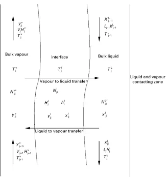
Nonequilibrium methods attempt to get around the difRculty of predicting efRciencies by replacing the equilibrium stage concept. Instead, they apply a transport phenomena approach for predicting mass transfer rates. Here, the bulk vapour and liquid phases are not at equilibrium with each other, but there is equilibrium at the interface between phases with a movement from the bulk phase through the interface (Figure 3). The net loss or gain of material and energy at the interface is expressed as transfer rates. The mass and energy transfer rates are depen-dent on the mass and energy transfer coefRcients for each phase which are in turn dependent on composi-tion and condicomposi-tions of each bulk phase and at the interface.
The correlations for the mass and heat transfer coefRcients and interface also take into account pack-ing or tray geometries for the actual column. The total mass and energy rates are calculated from inte-grating the mass and energy Suxes across the total interface surface.
Krishnamurthy and Taylor (1986) present and test a nonequilibrium model which includes rate equa-tions among the traditional MESH equaequa-tions. These include individual mass and energy balances in the vapour and the liquid and across the interface. An equilibrium equation exists for the interface only. The solution methods for these equations are the same as the global Newton methods.
The total mass transfer rates are added to an ex-panded set of the MESH equations called the MERQ equations. The new MERQ acronym stands for:
Material balances for each component}one for the bulk vapour, one for the bulk liquid and one across the interface.
Energy balance equations } one for the bulk va-pour, one for the bulk liquid and one across the interface.
Rate equations for mass transfer for all but one component } one from the interface to the bulk vapour and one from the bulk liquid to the inter-face, plus one energy transfer rate equation from the liquid to the vapour.
eQuilibrium equation at the interface only.
Outlook
Figure 3 Model of a nonequilibrium separation and mass transfer.
See also: II/ Distillation: Historical Development; Theory of Distillation; Vapour-Liquid Equilibrium: Correlation and Prediction; Vapour-Liquid Equilibrium: Theory.
Further Reading
Boston JF (1980) Inside-out algorithms for multicompo-nent separation process calculations. American Chem-ical Society Symposium Series No. 124: 135.
Brierley RJP and Smith RI (1979) DISTPACK }Using a combination of algorithms to solve difRcult distillation and absorption problems. Chemical Engineering Sym-posium Series No. 56: 89.
Friday JR and Smith BD (1964) An analysis of the equilib-rium stage separations problem}formulation and con-vergence. American Institute of Chemical Engineers Journal10: 689.
Holland CD (1981)Fundamentals of Multicomponent Dis-tillation. New York: McGraw-Hill.
Ketchum RG (1979) A combined relaxation}Newton method as a new global approach to the computation of thermal separation processes. Chemical Engineering Science34: 387.
Kister HZ (1992) Distillation Design. New York: McGraw-Hill.
Kister HZ (1995) Troubleshooting distillation simulation. Chemical Engineering Progress16(6): 63.
Krishnamurthy R and Taylor R (1986) Multicomponent mass transfer theory and applications. In Cheremisinoff NP (ed.)Handbook of Heat and Mass Transfer. Gulf Publishing Company.
Lockett MJ (1986)Distillation Tray Fundamentals. Cam-bridge, UK: Cambridge University Press.
Naphtali L and Sandholm DS (1971) Multicomponent sep-arations calculations by linearization. American Insti-tute of Chemical Engineers Journal17: 148.
Russell RA (1983) A Sexible and reliable method solves single-tower and crude-distillation-column problems. Chemical Engineering90(20): 53.
Taylor R, Wayburn TL and Vickery DJ (1987) The Devel-opment of Homotopy methods for the solution of se-paration process problems. International Chemical Engineering Symposium Series No. 104: B305. Wang JC and Henke GE (1996) Tridiagonal matrix