Haar Wavelet Matrices Designation in Numerical Solution of Ordinary Differential Equations

Haar Wavelet Matrices Designation in

Numerical Solution of Ordinary Differential

Equations

Phang Chang, Phang Piau

Abstract — Wavelet transforms or wavelet analysis is a recently developed mathematical tool for many problems. Wavelets also can be applied in numerical analysis. In this paper, we apply Haar wavelet methods to solve ordinary differential equations with initial or boundary condition known. To avoid the tedious calculations and to promote the study of wavelets to beginners, we proposed a simple way to perform the calculations for the matrix representation. The procedure applied in this paper is taking the Haar Series for the highest order of differential and integrate the series. Four numerical examples are shown which including first, second, higher order differential equations with constant and variable coefficients. The results show that the proposed way are quite reasonable when compare to exact solution.

Index Terms — Haar wavelet methods, matrix representation, ordinary differential equations, computer algebra system

I. INTRODUCTION

Wavelet transform or wavelet analysis is a recently developed mathematical tool for signal analysis. To date, wavelets have been applied in numerous disciplines such as image compression, data compression, denoising data and many more [1]. In numerical analysis, wavelets also serve as a Galerkin basis to solve partial differential equations. Wavelet analysis involves tedious calculations. Practically, the calculation is done by using software with certain commands or special toolboxes. It may make the beginner feel intimidate [2]. Meanwhile, Haar function always has been choose for educational purpose, especially in many papers or books written on topic of introduction to wavelets [3-4]. Due to the powerful of wavelets in plenty fields, there are many works, such as in [5-6] in promoting the study of wavelet even in undergraduate level.

Meanwhile in numerical analysis, wavelet based algorithms have become an important tools because of the properties of localization. One of the popular families of wavelet is Haar wavelets. Due to its simplicity, Haar wavelets

had become an effective tool for solving many problems, among that are Ordinary Differential Equations, ODEs and Partial Differential Equations, PDEs. In these works, the operator or matrix representation is expanded in a wavelet basis. Sometime, the works for writing up the operational matrices are quite tedious especially when ones intend to perform the calculation in high resolution. This will discourage the beginner to study how wavelet basis can be applied to solve differential equations, especially when in the works of encouraging the study of wavelets in undergraduate level which were done in [5-7].

Manuscript received July 22, 2008. This work was partially supported in part by the University Tun Hussein Onn Malaysia under Short Term Grant vot 0356 .

Phang Chang is with the Centre of Science Studies, University Tun Hussein Onn Malaysia, UTHM. 86400 Batu Pahat, Johor, Malaysia (phone: 607-4537973 ; fax: 607-4536051; e-mail: pchang@ uthm.edu.my).

Phang Piau is with Department of Computational Science and Mathematics, Faculty of Computer Science and Information Technology, University Malaysia Sarawak, UNIMAS, 94300 Kota Samarahan, Sarawak, Malaysia. (e-mail: [email protected]).

In solving ordinary differential equations by using Haar wavelet related method, Chen and Hsiao [8-9] had derived an operational matrix of integration based on Haar wavelet. Lepik [10] had solved higher order as well as nonlinear ODEs by using Haar wavelet method. There are discussions by other researchers [11-13]. We are not going to compare with these distinguish scholars, but intend to come out with a simple procedure to solve ordinary differential equations which make use of the power of wavelets. With this, we hope that even for an undergraduate student can also perform the numerical calculation by using wavelets as a tool in order to solve ordinary differential equation problems without using any complicated algorithm but sufficient with the help of computer algebra system or Excel. With this, it is hoped that it will encourage the study of wavelet in undergraduate level.

II. HAARWAVELET

Haar wavelet is the simplest wavelet. Haar transform or Haar wavelet transform has been used as an earliest example for orthonormal wavelet transform with compact support. The Haar wavelet transform is the first known wavelet and was proposed in 1909 by Alfred Haar. The Haar function can be described as a step function ψ(x)and in Fig. 1 as follows :

(1) ⎪

⎩ ⎪ ⎨ ⎧

≤ ≤ −

≤ ≤ =

otherwise 0

1 5 . 0 1

5 . 0 0 1

)

( x

x x

ψ

1

0

-1

0 1/2 1

This is also called mother wavelet. In order to perform wavelet transform, Haar wavelet uses translations and dilations of the function, i.e. the transform make use of following function

ψ(x)=ψ(2jx−k) (2) Translation / shifting ψ(x)=ψ(x−k)

Dilation / scaling ψ(x)=ψ(2jx)

where this is the basic works for wavelet expansion.

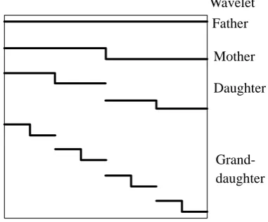
With the dilation and translation process as in Eq.(2), ones can easily obtain father wavelet, daughter wavelet, granddaughter wavelet and so on as in fig. 2.

Wavelet Father Mother Daughter

[image:2.595.70.261.215.373.2]

Grand-daughter

Fig. 2 Haar Wavelet (up to 2 resloution levels) In the matrix form, the Haar matrix for resolution up to 2 levels is given below :

⎟ ⎟ ⎟ ⎟ ⎟ ⎟ ⎟ ⎟ ⎟ ⎟ ⎟

⎠ ⎞

⎜ ⎜ ⎜ ⎜ ⎜ ⎜ ⎜ ⎜ ⎜ ⎜ ⎜

⎝ ⎛

− −

− −

− − −

−

− − − −

1 1 0 0 0 0 0 0

0 0 1 1 0 0 0 0

0 0 0 0 1 1 0 0

0 0 0 0 0 0 1 1

1 1 1 1 0 0 0 0

0 0 0 0 1 1 1 1

1 1 1 1 1 1 1 1

1 1 1 1 1 1 1 1

The pattern of the Haar wavelet undergo translation and dilation process and its matrix pattern are observed when the Haar wavelet been used in solving ordinary differential equations.

There are few important characteristics of Haar wavelet. First, it is a piecewise constant functions. Second, it is the simplest orthonormal wavelets, (Not all wavelets are orthonormal !) Third, it has the compact support [0, 1]. The first and third characteristics made Haar wavelet cannot be applied directly to solve ODE . The piecewise constant function means it is actually not continuous, and thus it cannot be differentiated in the points of discontinuity.

There is two possibilities to overcome these problems. One way is to regularize the piecewise constant Haar function using interpolation splines. However, this is not easy to do, thus the simplicity of Haar wavelet get loss. We did not apply this way in our work.

The second way is proposed by Chen and Hsiao [8], which is expand the highest derivative in the differential equation into Haar series. Other derivatives are obtained through integrations. The whole system is discretized by collocation method. The collocation method here is actually refer to segmentation process.

III. HAAR WAVELET METHOD FOR ORDINARY DIFFERENTIAL EQUATIONS

For solving linear ordinary differential equation with nth order, say

) ( ) ( )

( )

( ₂ ( 1)

) (

1y x A y x A y x f x

A n + n− +"+ _n = , where x∈

[ ]

A,B and initial conditions

) (

) 1 (

A

yn− , y(n−2)(A)",y(A) are known. We follow the work done by Lepik [10]. Say we intend to do until j level of resolution, hence we let . The interval

) 2 ( 2 j

m=

[ ]

A,B will be divided into msubintervals, hence

m A B

x= −

Δ and the matrices are in the dimension of m×m.

Here we suggest the step by step procedures for easy understanding. Mainly, there are 5 steps as shown in the procedure as follow.

Procedure:

Step 1: Let where h is haar matrix and is the wavelet coefficients.

∑

= = m i

i i n _{x ah x}

y

1 )

(

) ( )

(

i

a

Step 2: Obtain appropriate order of v y(x)by using

∑

∑

=

− −

=

+

− + −

= m i

v n

v i

v n i

v _{x aP x x A y}

y

1

1

0

) ( 0 ,

) (

) ( ! 1 )

( )

(

σ

σ σ

σ

Step 3: Replace y(n)(x) and all the value of y(v)(x) into the problem.

Step 4: Calculate the wavelet coefficients, ai. Step 5: Obtain the numerical solution fory(x).

Step 2 is the key procedure where matrix will be counted. If ones intend to do the calculation until level j of resolution, ones will obtain the matrix (let

) (

, x

Pn−vi

) (

, x

Pn−vi

α = −v

1 3α 5α 7α . . . (2m-1)α 1 3α 5α... (m-1)α

. . .

1 3α...( -1)α

Level 0 0 1 1 2 2 2 2 1 3α

1

3 1 Cα

α! (2m)α

m

2

represent elements which need to count

represent elements with the same value in same level Fig. 3: Designation of matrix P.

The pattern of design of the matrices P is similar to Haar wavelet. For calculation of P matrices, we focus on the elements need to be counted as shown in fig. 3. Here, we suggest the following algorithm for counting the elements which are required.

Algorithm :

⎥⎦ ⎤ ⎢⎣

⎡ _{+ −} α_{− −} α

α

α (2 ) ( (2 2 1)) 2( (2 1)) 1 ! 1 l C l m C m L v n− = α j

L=0,1,2,", (Level of Haar wavelet)

) 2 ( 2 , , 3 , 2 ,

1 m_L

l= "

and where C=B−A

In the matrix P shown in the fig 3, we factored out the common factor _α

α

α!(2 ) 1

m C

for all the elements in the matrix which we calculated using the algorithm above, for the reason of simplicity.

The good thing here is we need to obtain the matrix , or and so on for certain level of wavelet once only, and the same matrix can be stored and to be used for other different ODE if there is , or and so on needed to be obtained in this Step 2 if the interval of the problem and the level of resolution is same.

1

P

2

P

1

P P₂

IV. NUMERICAL EXAMPLES

Three examples are shown. All the calculation is done by using 3 levels of Haar wavelet.

Example 1:

Solve the equation y′′(x)+y(x)=sinx+xcosx,

] 1 , 0 [ ∈

x with y(0)=1, y′(0)=1. Exact solution :

) cos sin ( 4 1 sin 4 5 cos )

(x x x x2 x x x

y = + + −

By using

Step 1 :

∑

= = ′′ m

i i ih x

a x y 1 ) ( ) (

Step 2:

∑

∑

= − − = − + = m i i

iP x x y

a x y 1 1 0 2 0 ) ( 0 ,

2 ( 0)

! 1 ) ( ) ( σ σ σ σ

∑

= + + = m i i

iP x x

a

1 ,

2 ( ) 1

Step 3 : Hence, we get

x x x x y x

y′′( )+ ( )=sin + cos

x x x x x P a x h a m i i i m i i

i ( ) ( ) 1 sin cos

1 , 2 1 + = + + +

∑

∑

= =

[

h x P x

]

x x x x

a

m

i

i i

i + = + − −

∑

= 1 cos sin ) ( ) ( 1 , 2

The matrix P is shown below.

⎟ ⎟ ⎟ ⎟ ⎟ ⎟ ⎟ ⎟ ⎟ ⎟ ⎟ ⎟ ⎟ ⎟ ⎟ ⎟ ⎟ ⎟ ⎟ ⎟ ⎟ ⎟ ⎟ ⎟ ⎠ ⎞ ⎜ ⎜ ⎜ ⎜ ⎜ ⎜ ⎜ ⎜ ⎜ ⎜ ⎜ ⎜ ⎜ ⎜ ⎜ ⎜ ⎜ ⎜ ⎜ ⎜ ⎜ ⎜ ⎜ ⎜ ⎝ ⎛ 7 1 7 1 7 1 7 1 7 1 7 1 7 1 7 1 31 23 3 1 31 23 3 1 31 23 3 1 31 23 3 1 127 119 103 79 7 5 3 1 127 119 103 79 7 5 3 1 511 503 487 463 431 391 343 287 15 13 11 9 7 5 3 1 31 29 27 25 23 21 19 17 15 13 11 9 7 5 3 1 32 1 ! 2 1 2 2 2 2 2 2 2 2 2 2 2 2 2 2 2 2 2 2 2 2 2 2 2 2 2 2 2 2 2 2 2 2 2

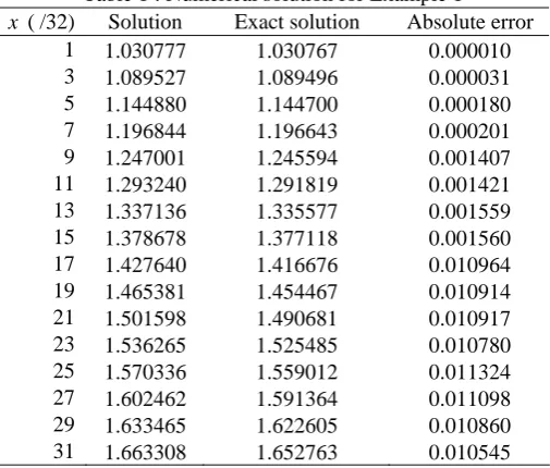
Step 4: Solving the system of linear equation. We obtain wavelet coefficients, ai.

[image:3.595.301.554.518.733.2]

Step 5: Obtain the numerical solution fory(x) as in Table 1. Table 1 : Numerical solution for Example 1

x ( /32) Solution Exact solution Absolute error

1 1.030777 1.030767 0.000010

3 1.089527 1.089496 0.000031

5 1.144880 1.144700 0.000180

7 1.196844 1.196643 0.000201

9 1.247001 1.245594 0.001407

11 1.293240 1.291819 0.001421

13 1.337136 1.335577 0.001559

15 1.378678 1.377118 0.001560

17 1.427640 1.416676 0.010964

19 1.465381 1.454467 0.010914

21 1.501598 1.490681 0.010917

23 1.536265 1.525485 0.010780

25 1.570336 1.559012 0.011324

27 1.602462 1.591364 0.011098

29 1.633465 1.622605 0.010860

31 1.663308 1.652763 0.010545

variable coefficient. Example 2:

Solve the equation y(4)(x)+xy(x)=16sin2x+xsin2x, ] 1 , 0 [ ∈

x with y(0)=0, y′(0)=2, y′′(0)=0, y′′′(0)=−8

Exact solution : y(x)=sin2x

By carry out Step 1 to 3, we obtain

[

h x xP x

]

x x x x x

a

m

i

i i

i 16sin2 sin2

3 4 2 ) ( )

( 2 4

1

,

4 + − = +

+

∑

=

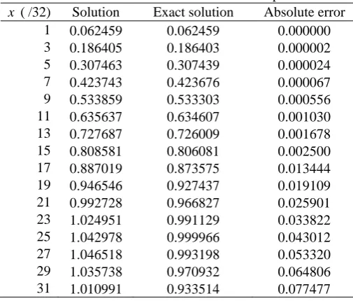
[image:4.595.304.547.35.463.2]

By carry out Step 4 to 5, we obtained the results as in Table 2. Table 2 : Numerical solution for Example 2

x ( /32) Solution Exact solution Absolute error

1 0.062459 0.062459 0.000000

3 0.186405 0.186403 0.000002

5 0.307463 0.307439 0.000024

7 0.423743 0.423676 0.000067

9 0.533859 0.533303 0.000556

11 0.635637 0.634607 0.001030

13 0.727687 0.726009 0.001678

15 0.808581 0.806081 0.002500

17 0.887019 0.873575 0.013444

19 0.946546 0.927437 0.019109

21 0.992728 0.966827 0.025901

23 1.024951 0.991129 0.033822

25 1.042978 0.999966 0.043012

27 1.046518 0.993198 0.053320

29 1.035738 0.970932 0.064806

31 1.010991 0.933514 0.077477

Example 3 involves ODE with exponential coefficients. The results is compare with the results obtained by series solution. Due to the behavior of exponential, we use a relatively small step size if compared to previous two examples, which is until 4 level of resolution.

Example 3:

Solve the equation y′(x)+exy(x)=x2, ] 1 , 0 [ ∈

x with y(0)=4.

Series solution : 3 4

12 1 4

4 )

(x x x x

y = − + + (up to first four nonzero terms only)

By carry out Step 1 to 3, we obtain =

+ ′(x) e y(x)

y x

[

]

x

m

i

i x i

ih x e P x x e

a ( ) ( ) 2 4

1

,

1 = −

+

∑

=

By carry out Step 4 to 5, we obtained the results as in Table 3 .

Table 3 : Numerical solution for Example 3

x ( /64) Solution Series solution Difference

1 3.936517 3.937504 0.000987

3 3.807570 3.812603 0.005034

5 3.674638 3.687980 0.013342

7 3.537674 3.563820 0.026146

Example 4:

Solve the equation y′′(x)+y(x)=sinx+xcosx,

] 1 , 0 [ ∈

x with y(0)=1, y(1)=1.667433.

Exact solution : ( sin cos )

4 1 sin 4 5 cos )

(x x x x2 x x x

y = + + −

= +

′(x) e y(x)

y x

[

]

x

m

i

i x i

ih x e P x x e

a ( ) ( ) 2 4

1

,

1 = −

+

∑

=

Compare to Example 1, slightly different consideration is done in Step 2 and 3.

Step 1 :

∑

= = ′′ m

i i ih x

a x y 1 ) ( ) (

Step 2:

∑

∑

= − − = − + = m i i

iP x x y

a x y 1 1 0 2 0 ) ( 0 ,

2 ( 0)

! 1 ) ( ) ( σ σ σ σ

∑

= ′ + + = m i i

iP x xy

a

1

0 ,

2 ( ) 1

where y0′ is unknown. y0′ can be found by consider

667433 . 1 ) 1 ( = y . 667433 . 1 ) 1 ( 1 ) 1 ( ) 1 ( 1 0 ,

2 + + ′ =

=

∑

= m

i i

iP y

a

y ,

Hence, (1) 0.667433

1 , 2 0

∑

= + − = ′ m i i iP a y

Step 3 : Fromy′′(x)+y(x)=sinx+xcosx, we obtain

x x x P a x x P a x h a m i m i i i i i m i i i cos sin 667433 . 0 ) 1 ( 1 ) ( ) ( 1 1 , 2 , 2 1 + = ⎥ ⎥ ⎦ ⎤ ⎢ ⎢ ⎣ ⎡ + − + + +

∑

∑

∑

= = =

Hence,

[

]

x x x x xP x P x h a m i i i i i 667433 . 0 1 cos sin ) 1 ( ) ( ) ( 1 , 2 , 2 − − + = − +

∑

=

[image:4.595.41.294.217.432.2]

By carry out Step 4 to 5, we obtained the results as in Table 4. Table 4 : Numerical solution for Example 4

x ( /32) Solution Exact solution Absolute error

1 1.036301 1.030767 0.005534

3 1.101311 1.089496 0.011815

5 1.159368 1.144700 0.014668

7 1.209068 1.196643 0.012425

9 1.257571 1.245594 0.011977

11 1.298038 1.291819 0.006219

13 1.336772 1.335577 0.001195

15 1.372508 1.377118 0.004610

17 1.415362 1.416676 0.001314

19 1.449621 1.454467 0.004846

21 1.482400 1.490681 0.008281

23 1.516283 1.525485 0.009202

25 1.549619 1.559012 0.009393

27 1.583481 1.591364 0.007883

29 1.616938 1.622605 0.005667

31 1.650668 1.652763 0.002095

V. CONCLUSION

[image:4.595.301.555.496.713.2]

procedure have been applied to use Haar wavelet method in solving ODEs. The result is comparable to the exact solution.

REFERENCES

[1] A.W. Galli, G.T. Heydt, and P.F. Ribeiro, “Exploring the power of wavelet analysis.” IEEE Computer Application in Power, Oct 1996, pp.37 – 41.

[2] M.N.O. Sadiku, C.M. Akujuobi, and R.C. Garcia, “An introduction to wavelets in electromagnetics.” Microwave Magazine, IEEE , vol. 6(2), June 2005, pp. 63 – 72.

[3] G.P. Nason, “A little introduction to wavelets.” Applied Statistical Pattern Recognition, IEEE Colloquium on 20 April 1999, pp.1 – 6. [4] E. Aboufadel and S. Schlicker, Discovering Wavelets, New York : John

Wiley & sons, Inc, 1999, pp. 12-18.

[5] M.C. Potter, J.L. Goldberg, E.F. Aboufadel, Advanced Engineering Mathematics. 3rd _{Ed. New York : Oxford University Press. pp. 670-699.}

[6] E. Aboufadel, S. Schlicker (2003) “Wavelets : Wavelets for undergraduates.” [Online]. Available:

http://www.gvsu.edu/math/wavelets/undergrad.htm

[7] P.V. O’Neil, Advanced Engineering Mathematics. 5th _{Ed. Thomson}

Brooks/Cole, 2003, pp. 841-854.

[8] Chen, C.F. and Hsiao C.H., “Haar wavelet method for solving lumped and distributed-parameter systems.” IEE Proc. Control Theory Appl. Vol 144, 1997, pp. 87-94

[9] Chen, C.F. and Hsiao C.H., “Wavelet approach to optimizing dynamic systems.” IEE Proc. Control Theory Appl. Vol 146, 1999, pp. 213-219. [10]Ülo Lepik, “Haar wavelet method for solving higher order differential

equations”

[11]Ülo Lepik, “Numerical solution of differential equations using Haar wavelets.” Mathematics and Computers in Simulation vol 68, 2005, pp. 127-143.

[12]Haydar Akca et.al., “Survey on wavelet transform and application in ODE and wavelet networks.” unpublished