An Upwind-mixed Finite Element Method with Moving Grids for Quasi-nonlinear Sobolev Equations

An Upwind-mixed Finite Element Method with

Moving Grids for Quasi-nonlinear Sobolev

Equations

Tongjun Sun, Ruirui Zheng

Abstract—An upwind-mixed finite element method with mov-ing grids is presented to simulate quasi-nonlinear Sobolev equations. This method is constructed by two methods. The upwind method is used to approximate the the convection term of Sobolev equations, meanwhile an expanded mixed finite element method is applied to discretize the diffusion term. The scalar unknown function and the adjoint vector function can be approximated simultaneously by this method. Optimal error estimates inL2

-norm are obtained for both the scalar unknown function and the adjoint vector function. Finally, numerical experiments are presented to illustrate the efficiency of this method.

Index Terms—Upwind method, mixed finite element method, moving grids, quasi-nonlinear Sobolev equations

I. INTRODUCTION

W

E consider the following quasi-nonlinear Sobolev equations

      

ut− ∇ ·

(

a(x, t)∇ut+b(x, t, u)∇u

)

+c(x, t, u)· ∇u

=f(x, t, u), x∈Ω, t∈(0, T], u(x, t) = 0, x∈∂Ω, t∈[0, T], u(x,0) =u0(x), x∈Ω,

(1) where Ω is a bounded subset of R2 _{with smooth} boundary ∂Ω, u0(x) and f(x, t, u) are known functions, the coefficients a(x, t), b(x, t, u),c(x, t, u) = (c1(x, t, u), c2(x, t, u))T_{satisfy the following condition:}

                              

0< a0≤a(x, t)≤a1, |∂a(x, t) ∂t | ≤a2,

0< b0≤b(x, t, u)≤b1,

|c(x, t, u)|= √

c2

1(x, t, u) +c22(x, t, u)≤c0,

|∂c(x, t, u)

∂u | ≤K1,

b(x, t, u),c(x, t, u), f(x, t, u)and∂c(x, t, u) ∂u are Lipschitz continuous with respect tou.

(2)

where a0, a1, a2, b0, b1, c0, K1 are positive constants. We assume that u(x, t) satisfy the smooth condition needed in the following analysis.

For time-changing localized phenomena, such as sharp fronts and layers, the finite element method with mov-ing grids [1]-[3] is advantageous over fixed finite element method. The reason is that the former treats the problem

This work was supported by the Natural Science Foundation of China under Grant 11271231 and 11301300.

The corresponding author T.J. Sun is in School of Mathematics, Shandong University, Jinan 250100, China, e-mail: [email protected]

R.R. Zheng is in Shandong Xiandai University, Jinan 250104, China.

with the finite element method on space domain by using different meshes and different basic functions at different time level so that it has the capability of self-adaptive local grid modification (refinement or unrefinement) to efficiently capture propagating fronts or moving layers. The paper [4] had combined this method with mixed finite element method to study parabolic problems.

Sobolev equations have important applications in many mathematical and physical problems, such as the percolation theory of the fluid flowing through the cracks [5], the transfer problem of the moisture in the soil [6], and the heat conduction problem in different materials [7]. Hence, there exists great and actual significance to discuss Sobolev equations in depth. Many papers had researched on numerical methods for Sobolev equations. More attentions were paid for treating the damping term∇·(a∇ut), which is a distinct

character of Sobolev equations different from parabolic e-quation. For example, time-stepping Galerkin methods were presented for nonlinear Sobolev equations in [8], [9]. In [10], [11], nonlinear Sobolev equations with convection term were researched by using finite difference streamline-diffusion method and discontinuous Galerkin method, respectively. Two new least-squares mixed finite element procedures were formulated for solving convection-dominated Sobolev equa-tions in [12]. In [13], two-grid methods for characteristic finite volume element approximations were considered for semi-linear Sobolev equations.

Mixed finite element method has been proven to be a powerful tool to numerically solve the fluid problems. It has an advantage of approximating the unknown function and its adjoint function simultaneously. The theoretical analysis and actual applications of mixed finite element method were discussed well, such as [14], [15], [16]. For the convection dominated equation, the solutions of standard finite element method often suffer from spurious oscillations. A variety of numerical techniques were put forward to solve this problem well, such as characteristic finite element method [17], [18], characteristic finite volume method [19]. The papers [20] and [21] introduced an upwind mixed covolume method and an upwind cell-centered difference method for the problem with diagonal diffusion tensor, respectively. Hughes and Brooks [22] proposed the streamline upwind Petrov-Galerkin method (SUPG) by adding an artificial diffusion in the streamline direction to diminish the oscillations. Johnson [23] and Johnson et al. [24] stabilized the SUPG method by adding another artificial diffusion in the crosswind direction to avoid overshooting and undershooting around the sharp fronts. In [25], an upwind-mixed method on changing meshes was considered for two-phase miscible flow in porous media.

IAENG International Journal of Applied Mathematics, 47:4, IJAM_47_4_15

This paper presents an upwind-mixed finite elemen-t meelemen-thod wielemen-th moving grids for quasi-nonlinear Sobolev equations. In Section II, this method is constructed by two methods. The convection term of Sobolev equations is approximated by the upwind method, and the diffusion term is discretized by an expanded mixed finite element method. This method can approximate simultaneously the scalar unknown function and the adjoint vector function effectively. Optimal error estimates in L2-norm are derived for both the scalar unknown function and the adjoint vector function in Section III. In Section IV, we present the results of numerical experiments, which confirm our theoretical results. We draw some conclusions in Section V.

Throughout the analysis, the symbol K will denote a generic constant, which is independent of mesh parameters

∆t,hand not necessarily the same at different occurrences.

II. UPWIND-MIXED METHOD WITH MOVING GRIDS

At first, we introduce some notations and basic assump-tions. The usual Sobolev spaces and norms are adopted onΩ. The inner product onL2_{(Ω)is denoted by(f, g) =}∫

Ωf gdx. Define the following two spaces

W =L2(Ω)/{φ≡constant onΩ}, V ={v∈H(div; Ω)| v·n= 0on ∂Ω}, wherenis the unit outward vector normal to∂Ω.

Let ∆tn _{>0 (n = 1,2,· · · , N}∗_{) denote different}

time-step size such thatT =

N∑∗

n=1

∆tn andtn =

n

∑

k=1

∆tk. We take

∆t= max

n ∆t

n_{. We assume that the time-step size∆t}n _do

not change too rapidly, that is, there exist positive constants λ_∗ andλ∗ which are independent ofnand∆t such that

λ_∗≤ ∆t

n

∆tn−1 ≤λ

∗_{. (3)}

For a given function g(x, t),we denote gn _{=g(x, t}n_).

At each time level tn_{, we construct a quasi-uniform}

partition Kn

h = {e

n

i} of Ω for the mixed finite element

space. And we assumehn _{be the diameter of e}n

i ∈Khn and

∆tn_=O(hn_{).We takeh= max}

n h

n_{. LetW}n

h×V

n

h ⊂W×V

and divVn

h =Whndenote the ”lowest-order” Raviart-Thomas

spaces. That is to say, on each elementen

i ∈Khn,Whn is the

space of functions which are constant and Vn

h is the space

of vector valued functions whose components are continuous and linear. The degrees of freedom of a function vn ∈V_hn correspond to the values of vn·γ at the midpoints of∂en_i. Here,∂en_i is the side ofen_i andγis the unit outward vector normal to ∂en

i.

By introducing variables z˜=−∇u,z =bz˜+az˜t,g =

cu= (c1u, c2u)T _{= (g1, g2)}T _{and c(¯ x, t, u) = (}∂c1

∂u, ∂c2

∂u)

T_,

we can rewrite the first equation in (1) as

ut+∇ ·z+∇ ·g+u¯c(u)·˜z=f(u). (4)

Here, we utilize the so-called ”expanded” mixed finite ele-ment method, proposed by Arbogast, Wheeler and Yotov[26], which gives a gradient approximation z˜and an approxima-tion z to the diffusion term.

Then, the weak formula of (4) is

      

(ut, w) + (∇ ·z, w) + (∇ ·g, w)

+(uc(¯u)·z˜, w) = (f(u), w), ∀w∈W,

(z˜,v) = (u,∇ ·v), ∀v∈V,

(z,v) = (b(u)z˜+az˜t,v), ∀v∈V.

(5)

The upwind-mixed finite element method with moving grids is presented as follows: at each time leveln, ∀wn _∈

Wn

h,vn∈Vhn, findUn ∈Whn,Zn ∈Vhn such that

                                

(U

n_−Rn_Un−1

∆tn , w

n_{) + (∇ ·Z}n_{, w}n_{) + (∇ ·G}n_{, w}n₎

+(Un_c(¯Un_)·Z˜n_{, w}n_{) = (f(U}n_{), w}n_),

(Rn_Un−1_−Un−1_{, w}n_{) = 0,}

(Z˜n,vn_{) = (U}n_{,∇ ·v}n_),

(Zn_,vn_{) = (b(U}n_)Z˜n_+anZ˜ n

−RnZ˜n−1 ∆tn ,v

n_),

(an(RnZ˜n−1−Z˜n−1),vn) = 0.

(6) When different finite element spaces are used at time leveltn

andtn−1_{, the second and fifth equations of (6) give the L}2 -projection{Rn_Un−1_{, R}n_Z˜n−1_{}of the previous approximate}

solution{Un−1_,Z˜n−1_{}into the current finite element space} Wn

h ×Vhn. Then, this projection is used as initial value to

calculate{Un_,Z˜n_{}in the first and third equations of (6). If}

the finite element spaces are same at time leveltn _andtn−1_, we know thatRn_Un−1_=Un−1_{, R}n_Z˜n−1_=Z˜n−1_.

In equation (6),Gn is constructed by the upwind method [25]. Since g = cu = 0 on ∂Ω, we set the integral average ofGn·γequal to zero on boundary edges. Suppose that elements e1 ande2 share an interior edge l, xl be the

midpoint of the edgel, andγlpoint frome1toe2. Then we adopt ([25])

Gn·γl=

{

Un e1(c(U

n−1_)·γ

l)(xl),if(c(Un−1)·γl)(xl)≥0,

U_en₂(c(Un−1)·γl)(xl),if(c(Un−1)·γl)(xl)<0,

where Un

e1 and U

n

e2 are the constant values of U

n _{on the}

elementse1 ande2, respectively.

III. ERROR ESTIMATES

In order to derive optimal error estimates, we need three projections. First, define ∏un ∈ W_hn,∏˜z˜n ∈ V_hn to be the L2-projection of un ∈ H1(Ω) and z˜n ∈ H(div,Ω)

respectively, which satisfy

{

(un_{, w}n_{) = (}∏_un_{, w}n_{), ∀w}n_∈Wn h,

(an_z˜n_,vn_{) = (a}n∏˜_z˜n_,vn_{), ∀v}n_∈Vn h.

(7)

Then, define πzn _{∈ V}n

h to be the π-projection of z

n _∈

H(div,Ω), which satisfies

(∇ ·(zn−πzn), wn) = 0, ∀ wn∈W_hn. (8)

According to [25], [27], these projections have the following approximate properties

      

∥un−∏un∥ ≤Khn,

∥z˜n₋∏˜_z˜n_∥+∥(z˜n₋∏˜_z˜n₎

t∥ ≤Khn,

∥zn−πzn∥ ≤Khn.

(9)

At time level tn, for ∀ wn ∈ W_hn, vn ∈ V_hn, we know

IAENG International Journal of Applied Mathematics, 47:4, IJAM_47_4_15

that the exact solutions satisfy                  (u

n_−un₋1

∆tn , w

n_{) + (∇ ·z}n_{, w}n_{) + (∇ ·g}n_{, w}n₎

+(un_c(¯un_)·z˜n_{, w}n_{) = (f(u}n_{), w}n_)−(ρn_{, w}n_),

(z˜n,vn) = (un,∇ ·vn),

(zn_,vn_{) = (b(u}n_)z˜n_+anz˜

n_−z˜n₋1

∆tn ,v

n_{) + (r}n_,vn_),

(10)

whereρn_=un

t −

un_−un−1

∆tn ,r

n_=an_(z˜n

t −

˜

zn_−z˜n−1

∆tn ).

Denote

ξu=U−

∏

u, ηu=u−

∏

u,

˜

ξz=Z˜− ˜

∏ ˜

z, η˜z= ˜z− ˜

∏ ˜ z,

ξz=Z−πz, ηz=z−πz.

Using the projections (7) and (8), we subtract (10) from (6) to get

                                       (ξ n

u−ξ

n₋1

u

∆tn , w

n_{) + (∇ ·ξ}n z, w

n_{) + (∇ ·(G}n_−gn_{), w}n₎

+(Unc(¯Un)·Z˜n, wn)−(unc(¯un)·z˜n, wn)

= (ρn, wn) + (f(Un)−f(un), wn) + (η

n u−ηnu−1

∆tn , w n_),

(ξ˜zn,vn) = (ξun,∇ ·vn),

(ξ_zn,vn) = (b(Un)Z˜n−b(un)z˜n,vn)−(rn,vn)

+(anZ˜

n_−Z˜n−1

∆tn ,v

n_{) + (η}n z,v

n₎

−(anz˜

n_−z˜n−1

∆tn ,v n

).

(11) Here, the last term of the first equation of (11) is related to the moving grids. If the grids don’t change, this term is equal to zero.

Taking wn _=ξn

u, vn=ξnz and vn=ξ˜zn sequentially in

(11) and adding together, we obtain

(ξ

n u−ξun−1

∆t , ξ

n

u) + (b(U

n_)Z˜n_−b(un_)z˜n_,ξ˜n z)

+(an

˜

Zn−Z˜n−1 ∆tn ,ξ˜

n z)−(a

nz˜

n_−z˜n₋1

∆tn ,ξ˜ n z)

= (f(Un_)−f(un_{), ξ}n

u) + (ρn, ξun) + (∇ ·(gn−Gn), ξun)

−(Un_c(¯Un_)·Z˜n_{, ξ}n

u) + (unc(¯ un)·z˜n, ξun)

+(rn_,ξ˜n

z)−(ηzn,ξ˜nz) + (

ηn u−ηnu−1

∆tn , ξ n u).

(12) Furthermore, we notice that

(I)

(b(Un)Z˜n−b(un)z˜n,ξ˜_zn) = (b(Un)ξ˜n_z,ξ˜n_z)−(b(Un)η˜_zn,ξ˜n_z)

+([b(Un)−b(un)]z˜n,ξ˜_zn),

(13)

(II)

(an

˜

Zn_−Z˜n−1

∆tn ,ξ˜ n z)−(an

˜

zn_−z˜n−1

∆tn ,ξ˜ n z)

= (an

˜

ξzn−ξ˜nz−1

∆tn ,ξ˜ n z)−(an

˜

ηnz−η˜nz−1

∆tn ,ξ˜ n z),

(14)

(III)

(Un_c(¯Un_)·Z˜n_{, ξ}n

u)−(unc(¯ un)·z˜n, ξun)

= ([ξn

u −ηun]¯c(Un)·Z˜n, ξnu) + (un[¯c(Un)−c(¯un)]·Z˜n, ξnu)

+(un_{c(¯ u}n_)·[ξ˜n

z−η˜nz], ξnu).

(15) The last second term in (14) is related to the moving grids. If the grids don’t change, this term is equal to zero.

We substitute (13)-(15) into (12) to yield

(ξ

n u −ξun−1

∆tn , ξ n

u) + (b(U n_)ξ˜n

z,ξ˜ n z) + (a

nξ˜zn−ξ˜nz−1

∆tn ,ξ˜ n z)

= (f(Un_)−f(un_{), ξ}n

u) + (ρn, ξnu) + (∇ ·(gn−Gn), ξun)

+(rn,ξ˜n_z)−(η_zn,ξ˜_zn) + ([η_un−ξn_u]¯c(Un)·Z˜n, ξn_u) −(un[¯c(Un)−c(¯un)]·Z˜n, ξ_un) + (b(Un)η˜_zn,ξ˜n_z)

+(η

n

u−η

n₋1

u

∆tn , ξ n u) + (u

n_{c(¯ u}n_)·[η˜n z−ξ˜

n z], ξ

n u)

+([b(un)−b(Un)]z˜n,ξ˜n_z) + (anη˜

n

z −η˜nz−1

∆tn ,ξ˜ n z) Def.

= T1+T2+· · ·+T12.

(16) Now, we turn to analyze each term in (16). First of all, for the first and third terms on the left-hand side, we have

(ξ

n u−ξun−1

∆tn , ξ n u)

= 1 2∆tn

{

[∥ξn_u∥2− ∥ξ_un−1∥2+∥ξ_un−ξ_un−1∥2

}

, (17)

(an

˜ ξn

z−ξ˜nz−1

∆tn ,ξ˜ n z)

≥ 1

2∆tn

{

[(anξ˜_zn,ξ˜n_z)−(an−1ξ˜_zn−1,ξ˜n_z−1)]

+a0∥ξ˜n_z−ξ˜n_z−1∥2 }

−a2 2 ∥

˜ ξn_z−1∥2.

(18)

Following from (16), (17) and (18), we derive

1 2∆tn

{

[∥ξ_un∥2− ∥ξn_u−1∥2+∥ξ_un−ξ_un−1∥2

}

+ (b(Un)ξ˜n_z,ξ˜n_z)

+ 1 2∆tn

{

[(anξ˜n_z,ξ˜n_z)−(an−1ξ˜_zn−1,ξ˜_zn−1)]

+a0∥ξ˜n_z−ξ˜_zn−1∥2 }

≤ a2 2 ∥

˜

ξ_zn−1∥2+T1+T2+· · ·+T12.

(19) By the Lipschitz continuity ofb,¯candf, some terms on the right-hand side of (19) can be estimated as follows:

T1≤K∥ξun∥2+Kh2, (20)

T2≤K∆tn∂ 2_u

∂t2 2

L2_(tn−1_,tn_;H1₎+K∥ξ

n u∥

2_{, (21)}

T4≤K∆tn∂ 2_u

∂t2 2

L2_(tn−1_,tn_;H1₎+

ε

10∥ ˜ ξzn∥

2

, (22)

T5≤K∥ηnz∥

2₊ ε

10∥ ˜

ξ_zn∥2, (23)

T6≤K∥ξn

u∥2+Kh2, (24)

T7≤K∥un_Z˜n_∥∥ξn

u∥+K∥ξun∥2≤K∥ξnu∥2, (25)

IAENG International Journal of Applied Mathematics, 47:4, IJAM_47_4_15

T8≤Kb1∥η˜zn∥2+

ε

10∥ ˜ ξnz∥2≤

ε

10∥ ˜

ξzn∥2+Kh2, (26)

T10≤ ε

10∥ ˜

ξnz∥2+Kh2+K∥ξun∥2, (27)

T11≤K∥ξunz˜

n_∥+ ε

10∥ ˜

ξ_zn∥2≤K∥ξn_u∥2+ ε 10∥

˜ ξ_zn∥2,

(28) whereεis a sufficiently small positive constant.

We apply the similar technique in [17] to considerT3. Let πgn_∈Vn

h denote theπ-projection of g n_{, i.e.}

(∇ ·(gn−πgn), wn) = 0, ∀wn ∈ W_hn. (29) Takingvn_=πgn_−Gn_{in the second equation of (11), then}

we have

(ξ˜n

z, πgn−Gn) = (∇ ·(gn−Gn), ξun)

so that

(∇ ·(gn−Gn), ξn_u) = (ξ˜n_z, πgn−Gn)

≤1 2(b(U

n_)ξ˜n z,ξ˜

n

z) +Kb−

1 0 ∥πg

n_−Gn_∥2_. (30)

Le l be the common interior edge between elements e1 ande2, and hl denote the length of this edge. Letγl denote

the unit vector normal tolandxldenote the midpoint of the

edge. By the property ofπ-projection [18], we see

∫

l

πgn·γlds=

∫

l

un(cn·γl)ds. (31)

Ifgn _{is smooth enough, by the midpoint rule of integration}

1

hl

∫

l

πgn·γlds−(c(un)·γl)un(xl) =O(h2l),

we derive

1

hl

∫

l

(πgn−Gn)·γlds

=un(xl)(c(un)−c(un−1))·γl

+un_(x

l)(c(un−1)−c(Un−1))·γl

+(un_(x

l)−Uen)c(Un−1)·γl+O(h2l).

(32)

Furthermore, ifun _{is smooth enough, we have}

|un_(x

l)−Uen| ≤ |ξun|+O(hn). (33)

Noticing that for∀v ∈Vh, the functionv is specified in

the interior of Ω and v ·γ is a constant on each edge of element e. From (31) to (33), we have

∥πgn−Gn∥2≤K∥ξ_un∥2+K{(∆t)2+h2}, (34) then

T3≤

1 2(b(U

n_)ξ˜n z,ξ˜

n

z) +Kb−

1 0

{

∥ξ_un∥2+ (∆t)2+h2}. (35)

Substituting (20)-(28) and (35) into (19), we obtain

1 2∆tn

{

[∥ξ_un∥2− ∥ξ_un−1∥2+∥ξn_u−ξ_un−1∥2

}

+1 2(b(U

n_)ξ˜n z,ξ˜

n z) +

a0

2∆tn∥ξ˜ n z−ξ˜

n₋1

z ∥

2

+ 1 2∆tn[(a

n_˜

ξzn,ξ˜ n z)−(a

n₋1_˜

ξnz−1,ξ˜ n₋1

z )]

≤ε 2∥

˜

ξn_z∥2+a2 2 ∥

˜

ξn_z−1∥2+K{∥ξn_u∥2+ (∆t)2+h2}

+K(∆tn)∂

2_u

∂t2 2

L2_(tn−1_,tn_;H1₎+T9+T12.

(36)

LetN be the time-step at which∥ξn

u∥is maximal, that is,

∥ξ_uN∥2= max

1≤n≤N∗∥ξ n u∥

2_.

Multiplying (36) by2∆tn and summing onn from1toN, we obtain

∥ξN

u∥2+

N

∑

n=1

∥ξn

u−ξun−1∥2∆tn+b0

N

∑

n=1

∥_ξ˜n z∥2∆tn

+a0

N

∑

n=1

∥_ξ˜n

z−ξ˜nz−1∥2+a0∥ξ˜Nz∥2

≤K{(∆t)2_+h2}₊ ∑N

n=1

{

K∥ξn

u∥2+ε∥ξ˜zn∥2

} ∆tn

+a2

N

∑

n=1

∥_ξ˜n−1

z ∥2∆tn+∥ξ0u∥2+a1∥ξ˜0z∥2

+2

N

∑

n=1

{ (η

n u−ηun−1

∆tn , ξ n u) + (a

nη˜nz−η˜nz−1

∆tn ,ξ˜ n z)

} ∆tn.

(37) Assuming that the grids change at most M times in the time interval[0, T], andM ≤M∗,whereM∗is independent ofhand∆t, we can get the following two analysis [3]:

2

N

∑

n=1

(η

n

u−ηun−1

∆tn , ξ n u)∆t

n_≤K(M∗h)2₊1

4∥ξ

N

u∥

2_,

(38)

2

N

∑

n=1

(anη˜

n

z−η˜nz−1

∆tn ,ξ˜ n z)∆t

n_≤Kh2_+ε

N

∑

n=1

∥_ξ˜n z∥

2_∆tn_.

(39) Substituting (38) and (39) into (37), we find

3 4∥ξ

N

u∥

2₊

N

∑

n=1

∥ξn_u−ξ_un−1∥2∆tn+b0

N

∑

n=1

∥_ξ˜n z∥

2_∆tn

+a0

N

∑

n=1

∥_ξ˜n

z−ξ˜nz−1∥2+a0∥ξ˜Nz∥2

≤K{(∆t)2+h2+ (M∗h)2}+∥ξu0∥2+a1∥ξ˜z0∥2

+

N

∑

n=1

{

K∥ξn

u∥2+ 2ε∥ξ˜nz∥2+a2∥ξ˜zn−1∥2

} ∆tn_.

(40) Choosing 0 < ε < b0/2 and using the discrete Gronwall’s lemma, we have

max

n ∥ξ

n u∥

2_≤K{_(∆t)2_+h2_{+ (M}∗_h)2}_{, (41)}

and

max

n ∥

˜ ξzn∥

2_≤

K{(∆t)2+h2+ (M∗h)2}. (42)

By the triangle inequality and (9), we obtain the following result:

Theorem 3.1: Assuming that the coefficients satisfy the condition (2), and the grids change at most M times in the time interval [0, T], M ≤ M∗ and u ∈ L2_(H1_{), u}

t ∈

L2_(H1_{), u}

tt∈L2(H1),then we derive

max

n ∥u

n_−Un_{∥ ≤K}{_{h+ ∆t+M}∗_h}_,

max

n ∥z˜

n_−Z˜n_{∥ ≤K}{_{h+ ∆t+M}∗_h}_,

where K and M∗ are positive constants independent of h and∆t.

IAENG International Journal of Applied Mathematics, 47:4, IJAM_47_4_15

IV. NUMERICAL EXAMPLE

In this section, we present numerical experiments to il-lustrate the efficiency of our upwind-mixed finite element method with moving grids. We consider the model (1) on

(x, t) ∈ [0,1]×[0,1], where a(x, t) = t2(x+ 0.25) + 0.25, b(x, t, u) = 0.005ut2_{(x+ 0.05), c(x, t) = 0.05t(x+}

1) + 1 and f(x, t, u) is chosen properly so that the exact solution is u=e−t_sinπx.

To compare the computations and show the convergence rate easily, we set h and ∆t change according to the following four cases:

Casei: Ift∈[0,0.4], seth= ∆t= 0.1; Ift∈(0.4,0.6], seth= ∆t= 0.05; Ift∈(0.6,1.0], seth= ∆t= 0.1 and calculate 40 steps in every time interval.

Case ii: If t ∈ [0,0.4], set h = ∆t = 0.05; If t ∈

(0.4,0.6], set h = ∆t = 0.025; If t ∈ (0.6,1.0], set h= ∆t= 0.05and calculate 80 steps in every time interval. Case iii: If t ∈ [0,0.4], set h = ∆t = 0.025; If t ∈

(0.4,0.6], set h = ∆t = 0.0125; If t ∈ (0.6,1.0], set h= ∆t= 0.025and calculate 160 steps in every time interval.

Case iv: If t ∈ [0,0.4], set h = ∆t = 0.0125; If t ∈

(0.4,0.6], set h= ∆t = 0.00625; If t∈(0.6,1.0], set h= ∆t= 0.0125and calculate 320 steps in every time interval. The numerical solutionsUn_,Z˜n_{are computed and theL}2 -norm error estimates ofUn_−un_,Z˜n_−z˜n _{are obtained, see}

[image:5.595.70.268.379.507.2]

Tables I and II below, respectively.

Table I. L2_{-norm error estimates of U}n_−un

time Casei Caseii Caseiii Caseiv

t=0.4 0.0454 0.0232 0.0117 0.0057 t=0.6 0.0250 0.0134 0.0064 0.0031 t=1.0 0.0289 0.0158 0.0079 0.0039

Table II. L2_{-norm error estimates ofZ˜}n_−z˜n

time Casei Caseii Caseiii Caseiv

t=0.4 0.0531 0.0303 0.0159 0.0068 t=0.6 0.0637 0.0348 0.0161 0.0074 t=1.0 0.0627 0.0384 0.0190 0.0093

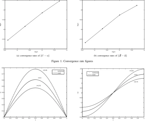
The convergence rates ofUn_−un_,Z˜n_−z˜n _{are given in}

Table III, which are also shown by Figure 1. From Fig. (a) and (b), we can see that the convergence rate of Un _−un

is one order and that of Z˜n_−z˜n _{is little smaller than one}

order at the beginning. But the convergence rateZ˜n_−z˜n_will

be close to one order whenhdecreases, which is consistent with the analysis in this paper.

Table III. Convergence rate ofL2_-norm

time Rates of∥un_−Un_{∥ Rates of∥z˜}n_−Z˜n_∥ i/ii ii/iii iii/iv i/ii ii/iii iii/iv t=0.4 0.9683 0.9857 1.0383 0.8082 0.9276 1.2178 t=0.6 0.9024 1.0620 1.0388 0.8718 1.1121 1.1300 t=1.0 0.8512 1.0072 1.0153 0.7074 1.0136 1.0352

For Case iv, we compare the exact solution u,z˜ with the approximate solution U,Z˜ at time t = 0.25,0.5,0.75

respectively, see Figure 2. From Fig. (c) and Fig. (d), we can see that the approximate solutions are very close to the exact solutions.

V. CONCLUSIONS

We have considered the upwind-mixed finite elemen-t meelemen-thod wielemen-th moving grids for quasi-nonlinear Sobolev

equations. This method is constructed by two methods. The convection term is approximated by the upwind method and the diffusion term is discretized by an expanded mixed finite element method. This method can simultaneously approx-imate the scalar unknown function and the adjoint vector function effectively. We have proved optimal error estimates in L2_{-norm for both the scalar unknown function and the} adjoint vector function, and presented numerical experiments to verify the validity of this method.

In this paper, the Sobolev equations we have considered are of quasi-nonlinear type. We can extend our method to the whole nonlinear Sobolev equations. The results for this case will be presented in a forthcoming paper.

ACKNOWLEDGMENT

The authors would like to thank the referees for their constructive comments leading to an improved presentation of this paper.

REFERENCES

[1] K. Miller and R. N. Miller, “Moving finite elements I,”SIAM Journal on Numerical Analysis, vol. 18, no. 6, pp. 1019-1032, 1981. [2] K. Miller, “Moving finite elements II,”SIAM Journal on Numerical

Analysis, vol. 18, no. 6, pp. 1033-1057, 1981.

[3] G. P. Liang and Z. M. Chen, “A full-discretization moving FEM with optimal convergence rate,”Mathematica Numerica Sinica, vol. 12, no. 3, pp. 318-337, 1990.

[4] D. Q. Yang, “The mixed finite element methods with moving grids for parabolic problems,”Mathematica Numerica Sinica, vol. 10, no. 3, pp. 266-271, 1988.

[5] G. I. Barenblatt, I. P. Zheltov and I. N. Kochina, “Basic concepts in the theory of seepage of homogenous liquids in fissured rocks,”Journal of Applied Mathematics and Mechanics, vol. 24, no. 5, pp. 1286-1303, 1960.

[6] D. M. Shi, “The nonlinear migration equation of the Moisture in Soil with initial boundary value problem,” Acta Mathematics Applicatae Sinica, vol. 13, no. 1, pp. 31-38, 1990.

[7] T. W. Ting, “A cooling process according to two-temperature theory of heat conduction,”Journal of Mathematical Analysis and Applications, Vol. 45, no. 1, pp. 23-31, 1974.

[8] R. E. Ewing, “Time-Stepping Galerkin methods for nonlinear Sobolev partial differential equations,” SIAM Journal on Numerical Analysis, vol. 15, no. 6, pp. 1125-1150, 1978.

[9] J. Zhu, “The finite element methods for nonlinear Sobolev equation,”

Northeastern Mathematical Journal, vol. 5, no. 2, pp. 179-196, 1989. [10] T. J. Sun and K. Y. Ma, “Finite difference streamline diffusion method

for quasilinear Sobolev equations,”Numerical Mathematics, A Journal of Chinese Universities, vol. 23, no. 4, pp. 340-356, 2001.

[11] T. J. Sun and D. P. Yang, “Error estimates for a discontinuous Galerkin method with interior penalties applied to nonlinear Sobolev equations,”

Numerical Methods for Partial Differential Equations, vol. 24, no. 3, pp. 879-896, 2008.

[12] J. S. Zhang, D. P. Yang and J. Zhu, “Two new least-squares mixed finite element procedures for convection-dominated Sobolev equations,”

Applied Mathematics, A Journal of Chinese Universities, vol. 26, no. 4, pp. 401-411, 2011.

[13] J. L. Yan and Z. Y. Zhang, “Two-grid methods for characteristic finite volume element approximations of semi-linear Sobolev equations,”

Engineering Letters, vol. 23, no. 3, pp. 189-199, 2015.

[14] P. A. Raviart and J. M. Thomas, “A mixed finite element method for second order elliptic problems,”in: Mathematical Aspects of the Finite Element Method, Lecture Notes in Mathematics,vol. 606, pp. 292-315, 1977.

[15] Jr. J. Douglas and J. E. Roberts, “Global estimates for mixed methods for second order elliptic equations,”Mathematics of computation, vol. 44, no. 169, pp. 39-52, 1985.

[16] M. C. Zhao, H. B. Guan and P. Yin, “A stable mixed finite element scheme for the second order elliptic problems,”IAENG International Journal of Applied Mathematics, vol. 46, no.4, pp. 545-549, 2016. [17] C. N. Dawson, T. F. Russell and M. F. Wheeler, “Some improved error

estimates for the modified method of characteristics,”SIAM Journal on Numerical Analysis, vol. 26, no. 6, pp. 1487-1512, 1989.

IAENG International Journal of Applied Mathematics, 47:4, IJAM_47_4_15

−4.5 −4 −3.5 −3 −2.5 −2 −6

−5.5 −5 −4.5 −4 −3.5

−log h

log e

(a) convergence rates of∥U−u∥

−4.5 −4 −3.5 −3 −2.5 −2

−5 −4.5 −4 −3.5 −3 −2.5

−log h

log e

[image:6.595.61.546.55.251.2]

(b) convergence rates of∥Z˜−z˜∥

Figure 1: Convergence rate figures

0 0.1 0.2 0.3 0.4 0.5 0.6 0.7 0.8 0.9 1

0 0.1 0.2 0.3 0.4 0.5 0.6 0.7 0.8

x

U

t=0.25

t=0.5

t=0.75

numerical exact

(c) comparinguwithU

0 0.1 0.2 0.3 0.4 0.5 0.6 0.7 0.8 0.9 1

−2.5 −2 −1.5 −1 −0.5 0 0.5 1 1.5 2 2.5

x

−ux

t=0.25

t=0.5

t=0.75 numerical

exact

(d) comparingz˜withZ˜

Figure 2: Compare figures for Caseiv at timet= 0.25,0.5,0.75

[18] Y. R. Yuan, “Characteristic finite element methods for positive semidefinite problem of two phase miscible flow in three dimensions,”

Chinese Science Bulletin, no. 22, pp. 2027-2032, 1996.

[19] L. Z. Qian and H. P. Cai, “Two-grid method for characteristics finite volume element of nonlinear convection-dominated diffusion Equations,”Engineering Letters,vol. 24, no. 4, pp. 399-405, 2016. [20] S. H. Chou and P. S. Vassilevski, “Mixed upwinding covolume

methods on rectangular grids for convectionCdiffusion problems,”SIAM Journal on Scientific Computing, vol. 21, no. 1, pp. 145-165, 1999. [21] S. H. Chou and P. S.Vassilevski, “An upwinding cell-centered methods

with piecewise constant velocity over covolume,”Numerical Methods for Partial Differential Equations, vol. 15, no. 1, pp. 49-62, 1999. [22] T. J. R. Hughes and A. N. Brooks, “Streamline upwind Petrov-Galerkin

formulations for convection-dominated flows with particular emphasis on the incompressible Navier-Stokes equations,”Computer methods in applied mechanics and engineering, vol. 32, no. 1-3, pp. 199-259, 1982. [23] C. Johnson, Numerical Solution of Partial Differential Equations by the Finite Element Method, Cambridge University Press, New York, 1987.

[24] C. Johnson, A. H. Schatz and L.B. Wahlbin, “Crosswing smear and pointwise errors in streamline diffusion finite element methods,”

Mathematics of Computation, vol. 49, no. 179, pp. 25-38, 1987. [25] H. L. Song and Y. R. Yuan, “An upwind-mixed method on changing

meshes for two-phase miscible flow in porous media,”Applied Numer-ical Mathematics, vol. 58, no. 6, pp. 815-826, 2008.

[26] T. Arbogast, M. Wheeler and I. Yotov, “Mixed finite elements for ellip-tic problems with tensor coefficients as cell-centered finite differences,”

SIAM Journal on Numerical Analysis, vol. 34, no. 2, pp. 828-852, 1997.

[27] M. F. Wheeler, “A prioriL2 _{error estimates for Galerkin} approxi-mations to parabolic partial differential equations,” SIAM Journal on Numerical Analysis, vol. 10, no. 4, pp. 723-759, 1973.

IAENG International Journal of Applied Mathematics, 47:4, IJAM_47_4_15

[image:6.595.53.548.57.471.2]