Suspended Sediment Simulation using Ann based Generalized Feed Forward Neural Network (GFF) and Multi Linear Regression Method (MLR)

© 2019, IRJET | Impact Factor value: 7.211 | ISO 9001:2008 Certified Journal

| Page 2794

“SUSPENDED SEDIMENT SIMULATION USING ANN BASED GENERALIZED

FEED FORWARD NEURAL NETWORK (GFF) AND MULTI LINEAR

REGRESSION METHOD (MLR)”

Mohd. Aamir

1

_{, Dr. S.K. Srivastava}

2

_{, Dr. Vikram Singh}

3

_{, Dr. D M Denis}

4

1

_{P.G Scholar ‘SHUATS’ Allahabad (U.P)}

2

_{Associate Professor Department of Irrigation & Drainage ‘SHUATS’ Allahabad (U.P)}

3

_{Assistant Professor Department of Soil Water Conservation Engineering ‘SHUATS’ Allahabad (U.P)}

4

_{Associate Professor Department of Irrigation & Drainage ‘SHUATS’ Allahabad (U.P)}

---***---Abstract -Estimates of sediment load are required in a wide spectrum of water resources engineering problems. The nonlinear nature of suspended sediment load series necessitates the utilization of nonlinear methods for simulating the suspended sediment load. In this study artificial neural networks (ANNs) and MLR method are employed to estimate the daily total suspended sediment load on Narmada river at Sankheda Gujarat. The simulations provided satisfactory simulations in terms of the selected performance criteria comparing well with conventional multi-linear regression. Similarly, the simulated sediment load hydrographs obtained by two ANN methods are found closer to the observed ones again compared with multi-linear regression.

Key Words: Sediment Simulation, GFF, MLR, Validation

1. INTRODUCTION

In many rivers, a major part of the sediment is transported in suspension. Recently, the importance of correct sediment prediction, especially in flood-prone areas, has increased significantly in water resources and environmental engineering. During the past few decades, a great deal of research has been devoted to the simulation and prediction of river sediment dynamics. This research has led to the formulation of a broad variety of methods and the development of a large number of models. The daily suspended sediment load (S) process is among one of the most complex nonlinear hydrological and environmental phenomena to comprehend, because it usually involves a number of interconnected elements. Studies have been conducted to reduce the complexities of the problem by developing practical techniques that do not require much algorithm and theory. In this way, classical models such as multi linear regression (MLR) and sediment rating curve (SRC) are widely used for suspended sediment modeling (Kisi et al 2005). The last decade has seen a tremendous growth in interest in the application of artificial neural networks (ANNs) to water resources and environmental problems.

2. REVIEW AND LITERATURE

Boukhrissa et al., (2013) investigated that sediment transport equations and direct measurement of sediment load were used for annual sediment load estimation. Sediment concentration data for long term was not available, due to this sediment rating curves and flux estimation were used widely. To improve the prediction capability of daily and annual basis sediment estimation various statistical models were used. El Kebir catchment has been chosen as the study area. Daily water discharge data was used as an input whereas daily suspended sediment data was used as a target based on different networks (cascade forward and FFBP) and algorithms (L-M and Bayesian regularization). The results showed that ANN model predicts the daily sediment load sediment yield annually more accurately and effectively.

Chen et al., (2013) developed a model for reliable runoff prediction using hourly rainfall data flow data from 3 rainfall stations namely Nanhe, Taiwu and Laii with one flow station as Sinpi in the Linbien basin using ANN approach. The linear and non-linear methods are incapable of predicting the runoff accurately as the hydrologic processes are complex in nature. 27 typhoons were occurred over a period of 2005-2009 according to the data records. To compare the performances of feed forward back propagation network and regression analysis various statistical parameters were used. It was found that FFBP performed much better as compared to the conventional regression analysis.

© 2019, IRJET | Impact Factor value: 7.211 | ISO 9001:2008 Certified Journal

| Page 2795

3. MATERIALS AND METHOD

3.1 General description of study area

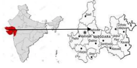
Sankheda is located on the banks of the Narmada River. It is located 55 km away from Vadodara lies between 22°10′15″ North and 73°34′45″East longitude. The soils found in South Gujarat and Saurashtra are predominantly clayey.

3.2 Rainfall & Climate

The climate here is tropical. When compared with winter, the summers have much more rainfall. The temperature here averages 27.2 °C. The average annual rainfall is 965 mm.

3.3 Data collection

The daily rainfall, runoff and sediment statistics of monsoon season (1 June to 30th September during the years 2004 to 2013 at Narmada basin in Sankheda, Gujarat station were obtained from CWC (Central Water Commission, Vadodara, Gujarat)S and metrological data from global weather data for SWAT(Soil and Water Assessment Tool).The daily meteorological data (i.e. discharge, sediment & rainfall) for monsoon period June 1st to September 30th from 2004 to 2013 for Sankheda, Gujarat were pre-processed in excel sheet and the data was divided into two parts i.e. 80 % training sets and 20 % testing sets.

3.4 Software used

Neuro solutions 5.0 for ANN (Artificial Neural Network) and Microsoft excel for MLR (Multi Linear Regression method).

3.5 Methodology

An ANN is a massively parallel-distributed information processing system that has certain performance characteristics resembling biological neural networks of the human brain. Ann has been developed as a generalization of mathematical models of human cognition or neural biology.

3.5.1 Generalised feed-forward network

A feed forward neural network is an artificial neural network wherein connections between the nodes do not form a cycle. As such, it is different from networks. The feed

[image:2.595.320.557.130.255.2]

forward neural network was the first and simplest type of artificial neural network devised.

[image:2.595.61.282.206.316.2]

Fig 3.2 Four layer feed forward neural network

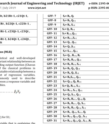
Table 3.1 output-input combinations for ANN based GFF models for sediment simulation at Sankheda area, Gujarat.

Model no. Input- Output Variable MLR- 1 St =a1 +b1 Rt

MLR- 2 St =a2 + c2 Rt-1 MLR - 3 St=a3 + b2 Qt MLR - 4 St= a4 + c2 Qt-1 MLR - 5 St= a5 + d1 St-1

MLR - 6 St= a6 + b3Rt + c3 Rt-1, MLR - 7 St= a7 +b4 Rt, b4 Qt

MLR -8 St= a8 + b24 Rt, + c24 Qt-1 MLR -9 St= a9 + b24 Rt, d2 St-1 MLR -10 St= a10 +b24 Rt-1 +c24 Qt MLR -11 St= a11+ c24 Rt-1 , c24 Qt-1 MLR -12 St= a12 + c24 Rt-1 , d3St-1 MLR -13 St= a13 + b24Qt , c24Qt-1 MLR -14 St=a14 + c24Qt , d4St-1 MLR -15 St= a15 + b24St-1 , d5Qt-1 MLR -16 St= a16 + b24Qt , b24Rt-1, c24Rt MLR -17 St= a17 + b24Rt, c24Rt-1, c24Qt-1 MLR -18 St=a18 + b24Rt, c24Rt-1, d6St-1 MLR -19 St= a19+ b24Rt, b24Qt,, c24Qt-1 MLR -20 St=a20 +b24 Rt, c24Qt ,d7St-1 MLR -21 St=a21 + b24Rt,c24St-1,, c24Qt-1 MLR -22 St= a22 + c24Qt-1, c24Qt, d8Rt-1 MLR -23 St= a23 + b16Qt, c17Rt-1, d9St-1 MLR -24 St= a24 + b17Rt-1, b17St-1, d10Qt-1 MLR -25 St=a25 + b18Qt, c18St-1, d11Qt-1

MLR -26 St=a26 + b19Rt, b19Rt-1 , c19Qt-1, d12Qt

© 2019, IRJET | Impact Factor value: 7.211 | ISO 9001:2008 Certified Journal

| Page 2796

MLR -28 St=a28 +b21Rt, b21Rt-1, c21Qt-1, c21St-1

MLR -29 St= a29 + b22Rt , b22Qt-1, c22St-1 , d14Qt

MLR - 30 St=a30 + b23Rt-1, c23Qt-1, c23Qt , d15St-1

MLR -31 St= a31 + b24Rt-1, b24Qt-1, c24Qt , c24St-1 , d16Rt

3.6 Multiple Linear Regression (MLR)

MLR is the simplest, statistical and well-developed representation of the time-invariant relationship between an input function and corresponding output function (Chavan and Ukrande, 2017). One of the classical problems in statistical analysis is to find a suitable relationship between a response variable and a set of regression variables. Regression analysis is commonly used to describe quantitative relationships between a response variable and one or more explanatory variables.

Where,

Y = Dependent variable;

α = Constant or intercept;

β1 = Slope (Beta coefficient) for X1;

X1 =First independent variable that is explaining the variance in Y;

β2 = Slope (Beta coefficient) for X2;

X2 = Second independent variable that is explaining the variance in Y;

p= Number of independent variables;

βp= Slope coefficient for Xp;

[image:3.595.164.544.44.477.2]

Xp= pth independent variable explaining the variance in Y.

Table 3.2 output-input combinations for MLR models for sediment simulation at Sankheda area, Gujarat.

Model no. Input- Output Variable GFF- 1 St = Rt

GFF- 2 St = Rt-1

GFF- 3 St= Qt

GFF- 4 St= Qt-1

GFF- 5 St= St-1

GFF- 6 St= Rt-1, Rt

GFF- 7 St= Rt, Qt

GFF- 8 St= Rt, Qt-1

GFF- 9 St= Rt, St-1

GFF- 10 St= Qt, Rt-1

GFF- 11 St= Rt-1 ,Qt-1

GFF- 12 St= Rt-1 ,St-1

GFF- 13 St= Qt , Qt-1

GFF- 14 St= Qt ,St-1

GFF- 15 St= St-1 , Qt-1

GFF- 16 St= Qt , Rt-1, Rt

GFF- 17 St= Rt, Rt-1, Qt-1

GFF- 18 St= Rt, Rt-1, St-1

GFF- 19 St= Rt, Qt,, Qt-1

GFF- 20 St= Rt, Qt ,St-1

GFF- 21 St= Rt,St-1,, Qt-1

GFF- 22 St= Qt-1, Qt, Rt-1

GFF- 23 St= Qt, Rt-1, St-1

GFF- 24 St= Rt-1, St-1, Qt-1

GFF- 25 St= Qt, St-1, Qt-1

GFF- 26 St= Rt, Rt-1 , Qt-1,Qt

GFF- 27 St= Rt, Rt-1 , Qt, St-1

GFF- 28 St= Rt, Rt-1 Qt-1, St-1

GFF- 29 St= Rt , Qt-1, St-1 , Qt

GFF- 30 St= Rt-1, Qt-1,Qt , St-1

GFF- 31 St= Rt-1, Qt-1,Qt , St-1 ,Rt

4. RESULT AND DISCUSSION

The model having higher values of correlation coefficient, coefficient of efficiency, coefficient of determination and lower value of mean square error is considered as the better fit model.

4.1 Suspended sediment modelling using Generalized Feed Forward Neural Network (GFF).

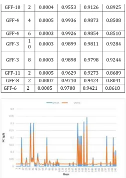
The values of performance evaluation indices for the simulated rainfall of the entire GFF model during testing and training are presented in table 4.1. GFF models GFF 1, GFF 2, GFF 3, GFF 4, GFF 6, GFF 8, GFF 9, GFF 10, GFF 12 and GFF 13 were selected for further analysis.

Table 4.1 Statistical indices for selected GFF model during

Model No.

N eu ro n

Testing

MSE r R2 _C.E

© 2019, IRJET | Impact Factor value: 7.211 | ISO 9001:2008 Certified Journal

| Page 2797

GFF-10 2 0.0004 0.9553 0.9126 0.8925

GFF-4 4 0.0005 0.9936 0.9873 0.8508

GFF-4 6 0.0003 0.9926 0.9854 0.8510

GFF-3 1₀ 0.0003 0.9899 0.9811 0.9284

GFF-3 8 0.0003 0.9898 0.9798 0.9244

[image:4.595.35.288.85.443.2] [image:4.595.310.566.186.719.2]

GFF-11 2 0.0005 0.9629 0.9273 0.8689 GFF-8 2 0.0007 0.9710 0.9424 0.8041 GFF-6 2 0.0005 0.9708 0.9421 0.8618

Fig 4.1 Comparison of observed and predicted suspended sediment by model 4 neuron 2 during the validation

[image:4.595.321.565.193.733.2] [image:4.595.36.289.495.648.2]

period.

Fig 4.1 Correlation between observed and predicted suspended sediment by model 4 neuron 2 during the

validation period

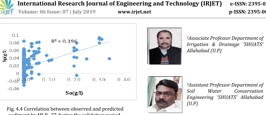
4.2Suspended sediment modelling using MLR (Multi Linear Regression) method

The observed (So) and predicted (Sp) SC values simulated by MLR models for testing period are compared in the form of SC graph and corresponding scatter-plot as shown in Figs.

4.2.1 to 4.1.21, which indicate that these models, in general, under predict the peak SC, which is confirmed by the scatter plots also. It was clearly indicated that the MLR models were not suitable for the prediction of SC for the study watersheds due to their very low values of CE and r during testing period.

Table 4.2 MLR sediment model during testing period 2004 – 2013.

Mode

l no. Regression equation

Testing

MSE CE R2

MLR 27

St=a26 + b19Rt, b19Rt-1 , c19Qt-1, d12Qt

0.003

5 0.0094 0.0094

MLR 29

St= a29 + b22Rt , b22Qt-1, c22St-1 , d14Qt

0.002

8 0.196 0.1962

MLR 30

St=a30 + b23Rt-1, c23Qt-1,c23Qt , d15St-1

0.002

8 0.194 0.1942 MLR

20 Sc24t=aQ20t ,d +b7S24t-1 Rt,

0.002

8 0.192 0.1917 MLR

23 S

t= a23 + b16Qt, c17Rt-1, d9St-1

0.002

9 0.164 0.1878 MLR

16 Sbt24= aRt-116, c + b2424RtQt ,

0.002

9 0.184 0.1839 MLR

7 SQtt= a7 +b4 Rt, b4

0.002

9 0.1800 0.18 MLR

19 Sbt24= aQt,19, c+ b24Q24t-1Rt,

0.002

9 0.18 0.1802 MLR

14 Sdt4=aSt-114 + c24Qt ,

0.002

9 0.178 0.1784 MLR

10 S+ct= a24 Q10t +b24 Rt-1

0.002

9 0.176 0.1761

[image:5.595.38.542.49.267.2]

© 2019, IRJET | Impact Factor value: 7.211 | ISO 9001:2008 Certified Journal

| Page 2798

Fig. 4.4 Correlation between observed and predicted sediment by MLR- 27 during the validation period.

5. CONCLUSION

The predicted suspended sediment using GFF models were found to be much closer to the observed values of sediment as compared to MLR Method for Shankheda, Gujarat the GFF model with input of rainfall, discharge was found to be the best for prediction of suspended sediment.It was clearly evident that MLR model fits very poorly for the dataset under study.

REFERENCES

[1] Kisi, O. 2005 “Suspended sediment estimation using

neuro-fuzzy and neural network approaches”, Hydrological Sciences Journal, 50(4): 683-696.

[2] Boukhrissa et al., (2013) J. Earth Syst. Sci. 122, No. 5,

October 2013, pp. 1303–1312 c Indian Academy of Sciences.

[3] Chen et al., (2013. Dual Artificial Neural Network for

Rainfall-Runoff Forecasting. Journal of Water Resource and Protection. 4: 1024-1028.

[4] Saemi, M. and Ahmadi, M. 2008. Integratin of genetic

algorithm and a co-active neuro- fuzzy inference system for permeability prediction from well logs data. Transp. Porous Media, 71: 273-288.

BIOGRAPHIES

1_{P.G Scholar ‘SHUATS’ Allahabad}

(U.P)

2_{Associate Professor Department of}

Irrigation & Drainage ‘SHUATS’ Allahabad (U.P)

3_{Assistant Professor Department of}

Soil Water Conservation