Constraints on cosmic strings using data from the first Advanced LIGO observing run

Constraints on cosmic strings using data from the first Advanced LIGO observing run.

B. P. Abbott,1 _{R. Abbott,}1 _{T. D. Abbott,}2 _{F. Acernese,}3,4 _{K. Ackley,}5 _{C. Adams,}6 _{T. Adams,}7 _{P. Addesso,}8 R. X. Adhikari,1 _{V. B. Adya,}9 _{C. Affeldt,}9 _{M. Afrough,}10 _{B. Agarwal,}11 _{M. Agathos,}12 _{K. Agatsuma,}13 N. Aggarwal,14_{O. D. Aguiar,}15 _{L. Aiello,}16,17 _{A. Ain,}18 _{P. Ajith,}19 _{B. Allen,}9,20,21 _{G. Allen,}11 _{A. Allocca,}22,23

P. A. Altin,24 A. Amato,25 A. Ananyeva,1 S. B. Anderson,1 W. G. Anderson,20S. Antier,26 S. Appert,1 K. Arai,1 _{M. C. Araya,}1 _{J. S. Areeda,}27_{N. Arnaud,}26,28 _{K. G. Arun,}29 _{S. Ascenzi,}30,17 _{G. Ashton,}9 _{M. Ast,}31

S. M. Aston,6 _{P. Astone,}32 _{P. Aufmuth,}21 _{C. Aulbert,}9 _{K. AultONeal,}33 _{A. Avila-Alvarez,}27 _{S. Babak,}34 P. Bacon,35_{M. K. M. Bader,}13_{S. Bae,}36_{P. T. Baker,}37,38_{F. Baldaccini,}39,40 _{G. Ballardin,}28_{S. W. Ballmer,}41 S. Banagiri,42 _{J. C. Barayoga,}1_{S. E. Barclay,}43_{B. C. Barish,}1_{D. Barker,}44_{F. Barone,}3,4 _{B. Barr,}43 _{L. Barsotti,}14

M. Barsuglia,35_{D. Barta,}45_{J. Bartlett,}44 _{I. Bartos,}46 _{R. Bassiri,}47 _{A. Basti,}22,23 _{J. C. Batch,}44 _{C. Baune,}9 M. Bawaj,48,40 _{M. Bazzan,}49,50 _{B. B´ecsy,}51 _{C. Beer,}9 _{M. Bejger,}52 _{I. Belahcene,}26 _{A. S. Bell,}43 _{B. K. Berger,}1 G. Bergmann,9 _{C. P. L. Berry,}53_{D. Bersanetti,}54,55_{A. Bertolini,}13 _{J. Betzwieser,}6_{S. Bhagwat,}41_{R. Bhandare,}56

I. A. Bilenko,57 _{G. Billingsley,}1_{C. R. Billman,}5 _{J. Birch,}6 _{R. Birney,}58 _{O. Birnholtz,}9 _{S. Biscans,}14_{A. Bisht,}21 M. Bitossi,28,23 _{C. Biwer,}41 _{M. A. Bizouard,}26 _{J. K. Blackburn,}1_{J. Blackman,}59 _{C. D. Blair,}60 _{D. G. Blair,}60 R. M. Blair,44 _{S. Bloemen,}61 _{O. Bock,}9 _{N. Bode,}9 _{M. Boer,}62 _{G. Bogaert,}62 _{A. Bohe,}34 _{F. Bondu,}63 _{R. Bonnand,}7 B. A. Boom,13 _{R. Bork,}1_{V. Boschi,}22,23 _{S. Bose,}64,18_{Y. Bouffanais,}35 _{A. Bozzi,}28_{C. Bradaschia,}23_{P. R. Brady,}20

V. B. Braginsky∗_,57 _{M. Branchesi,}65,66_{J. E. Brau,}67 _{T. Briant,}68 _{A. Brillet,}62 _{M. Brinkmann,}9_{V. Brisson,}26 P. Brockill,20 J. E. Broida,69 A. F. Brooks,1D. A. Brown,41 D. D. Brown,53 N. M. Brown,14 S. Brunett,1 C. C. Buchanan,2 _{A. Buikema,}14_{T. Bulik,}70 _{H. J. Bulten,}71,13 _{A. Buonanno,}34,72 _{D. Buskulic,}7 _{C. Buy,}35 R. L. Byer,47_{M. Cabero,}9 _{L. Cadonati,}73 _{G. Cagnoli,}25,74_{C. Cahillane,}1 _{J. Calder´on Bustillo,}73 _{T. A. Callister,}1 E. Calloni,75,4J. B. Camp,76 M. Canepa,54,55P. Canizares,61K. C. Cannon,77H. Cao,78J. Cao,79 C. D. Capano,9 E. Capocasa,35_{F. Carbognani,}28_{S. Caride,}80 _{M. F. Carney,}81_{J. Casanueva Diaz,}26_{C. Casentini,}30,17 _{S. Caudill,}20 M. Cavagli`a,10 _{F. Cavalier,}26 _{R. Cavalieri,}28_{G. Cella,}23 _{C. B. Cepeda,}1_{L. Cerboni Baiardi,}65,66_{G. Cerretani,}22,23 E. Cesarini,30,17_{S. J. Chamberlin,}82 _{M. Chan,}43_{S. Chao,}83 _{P. Charlton,}84_{E. Chassande-Mottin,}35_{D. Chatterjee,}20

B. D. Cheeseboro,37,38 _{H. Y. Chen,}85 _{Y. Chen,}59 _{H.-P. Cheng,}5 _{A. Chincarini,}55 _{A. Chiummo,}28 _{T. Chmiel,}81 H. S. Cho,86 _{M. Cho,}72 _{J. H. Chow,}24 _{N. Christensen,}69,62 _{Q. Chu,}60 _{A. J. K. Chua,}12 _{S. Chua,}68 A. K. W. Chung,87 _{S. Chung,}60 _{G. Ciani,}5_{R. Ciolfi,}88,89 _{C. E. Cirelli,}47_{A. Cirone,}54,55_{F. Clara,}44 _{J. A. Clark,}73

F. Cleva,62 _{C. Cocchieri,}10 _{E. Coccia,}16,17 _{P.-F. Cohadon,}68 _{A. Colla,}90,32 _{C. G. Collette,}91 _{L. R. Cominsky,}92 M. Constancio Jr.,15 _{L. Conti,}50 _{S. J. Cooper,}53_{P. Corban,}6 _{T. R. Corbitt,}2 _{K. R. Corley,}46_{N. Cornish,}93 A. Corsi,80_{S. Cortese,}28_{C. A. Costa,}15_{M. W. Coughlin,}69_{S. B. Coughlin,}94,95_{J.-P. Coulon,}62_{S. T. Countryman,}46

P. Couvares,1 _{P. B. Covas,}96 _{E. E. Cowan,}73 _{D. M. Coward,}60_{M. J. Cowart,}6_{D. C. Coyne,}1 _{R. Coyne,}80 J. D. E. Creighton,20 _{T. D. Creighton,}97 _{J. Cripe,}2 _{S. G. Crowder,}98 _{T. J. Cullen,}27 _{A. Cumming,}43 L. Cunningham,43 _{E. Cuoco,}28 _{T. Dal Canton,}76 _{S. L. Danilishin,}21,9 _{S. D’Antonio,}17 _{K. Danzmann,}21,9 A. Dasgupta,99 _{C. F. Da Silva Costa,}5 _{V. Dattilo,}28_{I. Dave,}56_{M. Davier,}26 _{D. Davis,}41 _{E. J. Daw,}100 _{B. Day,}73

S. De,41 _{D. DeBra,}47 _{J. Degallaix,}25 _{M. De Laurentis,}75,4_{S. Del´eglise,}68_{W. Del Pozzo,}53,22,23 _{T. Denker,}9 T. Dent,9 _{V. Dergachev,}34_{R. De Rosa,}75,4_{R. T. DeRosa,}6 _{R. DeSalvo,}101_{J. Devenson,}58 _{R. C. Devine,}37,38

S. Dhurandhar,18 _{M. C. D´ıaz,}97_{L. Di Fiore,}4 _{M. Di Giovanni,}102,89 _{T. Di Girolamo,}75,4,46 _{A. Di Lieto,}22,23 S. Di Pace,90,32 _{I. Di Palma,}90,32 _{F. Di Renzo,}22,23 _{Z. Doctor,}85 _{V. Dolique,}25 _{F. Donovan,}14 _{K. L. Dooley,}10 S. Doravari,9_{I. Dorrington,}95 _{R. Douglas,}43_{M. Dovale ´Alvarez,}53 _{T. P. Downes,}20 _{M. Drago,}9_{R. W. P. Drever}♯_,1

J. C. Driggers,44_{Z. Du,}79 _{M. Ducrot,}7 _{J. Duncan,}94_{S. E. Dwyer,}44 _{T. B. Edo,}100 _{M. C. Edwards,}69 _{A. Effler,}6 H.-B. Eggenstein,9_{P. Ehrens,}1_{J. Eichholz,}1_{S. S. Eikenberry,}5_{R. A. Eisenstein,}14 _{R. C. Essick,}14_{Z. B. Etienne,}37,38

T. Etzel,1_{M. Evans,}14 _{T. M. Evans,}6_{M. Factourovich,}46_{V. Fafone,}30,17,16 _{H. Fair,}41 _{S. Fairhurst,}95 _{X. Fan,}79 S. Farinon,55 _{B. Farr,}85_{W. M. Farr,}53 _{E. J. Fauchon-Jones,}95_{M. Favata,}103_{M. Fays,}95_{H. Fehrmann,}9 _{J. Feicht,}1 M. M. Fejer,47_{A. Fernandez-Galiana,}14_{I. Ferrante,}22,23 _{E. C. Ferreira,}15_{F. Ferrini,}28_{F. Fidecaro,}22,23 _{I. Fiori,}28 D. Fiorucci,35 _{R. P. Fisher,}41 _{M. Fitz-Axen,}42 _{R. Flaminio,}25,104 _{M. Fletcher,}43_{H. Fong,}105_{P. W. F. Forsyth,}24

S. S. Forsyth,73 _{J.-D. Fournier,}62 _{S. Frasca,}90,32 _{F. Frasconi,}23 _{Z. Frei,}51 _{A. Freise,}53 _{R. Frey,}67 _{V. Frey,}26 E. M. Fries,1 _{P. Fritschel,}14 _{V. V. Frolov,}6 _{P. Fulda,}5,76 _{M. Fyffe,}6 _{H. Gabbard,}9 _{M. Gabel,}106_{B. U. Gadre,}18 S. M. Gaebel,53 _{J. R. Gair,}107 _{L. Gammaitoni,}39 _{M. R. Ganija,}78 _{S. G. Gaonkar,}18 _{F. Garufi,}75,4 _{S. Gaudio,}33 G. Gaur,108_{V. Gayathri,}109 _{N. Gehrels}†_,76 _{G. Gemme,}55 _{E. Genin,}28 _{A. Gennai,}23 _{D. George,}11_{J. George,}56 L. Gergely,110_{V. Germain,}7 _{S. Ghonge,}73_{Abhirup Ghosh,}19 _{Archisman Ghosh,}19,13 _{S. Ghosh,}61,13_{J. A. Giaime,}2,6

J. M. Gonzalez Castro,22,23_{A. Gopakumar,}111 _{M. L. Gorodetsky,}57 _{S. E. Gossan,}1_{M. Gosselin,}28 _{R. Gouaty,}7 A. Grado,112,4_{C. Graef,}43 _{M. Granata,}25 _{A. Grant,}43 _{S. Gras,}14 _{C. Gray,}44 _{G. Greco,}65,66 _{A. C. Green,}53 P. Groot,61 _{H. Grote,}9 _{S. Grunewald,}34_{P. Gruning,}26 _{G. M. Guidi,}65,66 _{X. Guo,}79 _{A. Gupta,}82 _{M. K. Gupta,}99

K. E. Gushwa,1_{E. K. Gustafson,}1 _{R. Gustafson,}113_{B. R. Hall,}64 _{E. D. Hall,}1 _{G. Hammond,}43 _{M. Haney,}111 M. M. Hanke,9 _{J. Hanks,}44 _{C. Hanna,}82 _{M. D. Hannam,}95 _{O. A. Hannuksela,}87 _{J. Hanson,}6 _{T. Hardwick,}2

J. Harms,65,66 _{G. M. Harry,}114 _{I. W. Harry,}34 _{M. J. Hart,}43 _{C.-J. Haster,}105 _{K. Haughian,}43 _{J. Healy,}115 A. Heidmann,68 _{M. C. Heintze,}6_{H. Heitmann,}62 _{P. Hello,}26_{G. Hemming,}28 _{M. Hendry,}43_{I. S. Heng,}43 _{J. Hennig,}43

J. Henry,115A. W. Heptonstall,1 M. Heurs,9,21 S. Hild,43 D. Hoak,28 D. Hofman,25 K. Holt,6 D. E. Holz,85 P. Hopkins,95 _{C. Horst,}20 _{J. Hough,}43 _{E. A. Houston,}43 _{E. J. Howell,}60 _{Y. M. Hu,}9 _{E. A. Huerta,}11 _{D. Huet,}26 B. Hughey,33 _{S. Husa,}96 _{S. H. Huttner,}43 _{T. Huynh-Dinh,}6 _{N. Indik,}9 _{D. R. Ingram,}44_{R. Inta,}80_{G. Intini,}90,32 H. N. Isa,43_{J.-M. Isac,}68 _{M. Isi,}1_{B. R. Iyer,}19_{K. Izumi,}44_{T. Jacqmin,}68_{K. Jani,}73_{P. Jaranowski,}116_{S. Jawahar,}117

F. Jim´enez-Forteza,96 _{W. W. Johnson,}2_{D. I. Jones,}118 _{R. Jones,}43 _{R. J. G. Jonker,}13_{L. Ju,}60 _{J. Junker,}9 C. V. Kalaghatgi,95_{V. Kalogera,}94_{S. Kandhasamy,}6_{G. Kang,}36_{J. B. Kanner,}1 _{S. Karki,}67_{K. S. Karvinen,}9

M. Kasprzack,2 _{M. Katolik,}11 _{E. Katsavounidis,}14_{W. Katzman,}6 _{S. Kaufer,}21_{K. Kawabe,}44 _{F. K´ef´elian,}62 D. Keitel,43 _{A. J. Kemball,}11 _{R. Kennedy,}100 _{C. Kent,}95 _{J. S. Key,}119_{F. Y. Khalili,}57 _{I. Khan,}16,17 _{S. Khan,}9

Z. Khan,99 _{E. A. Khazanov,}120_{N. Kijbunchoo,}44 _{Chunglee Kim,}121_{J. C. Kim,}122 _{W. Kim,}78 _{W. S. Kim,}123 Y.-M. Kim,86,121 _{S. J. Kimbrell,}73 _{E. J. King,}78 _{P. J. King,}44 _{R. Kirchhoff,}9 _{J. S. Kissel,}44 _{L. Kleybolte,}31

S. Klimenko,5_{P. Koch,}9 _{S. M. Koehlenbeck,}9 _{S. Koley,}13 _{V. Kondrashov,}1_{A. Kontos,}14_{M. Korobko,}31 W. Z. Korth,1 _{I. Kowalska,}70 _{D. B. Kozak,}1_{C. Kr¨amer,}9 _{V. Kringel,}9_{B. Krishnan,}9 _{A. Kr´olak,}124,125_{G. Kuehn,}9

P. Kumar,105 _{R. Kumar,}99 _{S. Kumar,}19_{L. Kuo,}83 _{A. Kutynia,}124_{S. Kwang,}20_{B. D. Lackey,}34_{K. H. Lai,}87 M. Landry,44 R. N. Lang,20 J. Lange,115B. Lantz,47 R. K. Lanza,14 A. Lartaux-Vollard,26P. D. Lasky,126 M. Laxen,6 _{A. Lazzarini,}1 _{C. Lazzaro,}50_{P. Leaci,}90,32 _{S. Leavey,}43 _{C. H. Lee,}86_{H. K. Lee,}127 _{H. M. Lee,}121 H. W. Lee,122 _{K. Lee,}43 _{J. Lehmann,}9 _{A. Lenon,}37,38 _{M. Leonardi,}102,89 _{N. Leroy,}26 _{N. Letendre,}7 _{Y. Levin,}126

T. G. F. Li,87 A. Libson,14 T. B. Littenberg,128 J. Liu,60 R. K. L. Lo,87 N. A. Lockerbie,117 L. T. London,95 J. E. Lord,41 _{M. Lorenzini,}16,17_{V. Loriette,}129_{M. Lormand,}6 _{G. Losurdo,}23 _{J. D. Lough,}9,21 _{C. O. Lousto,}115 G. Lovelace,27_{H. L¨uck,}21,9 _{D. Lumaca,}30,17_{A. P. Lundgren,}9 _{R. Lynch,}14 _{Y. Ma,}59_{S. Macfoy,}58 _{B. Machenschalk,}9

M. MacInnis,14 _{D. M. Macleod,}2 _{I. Maga˜na Hernandez,}87 _{F. Maga˜na-Sandoval,}41 _{L. Maga˜na Zertuche,}41 R. M. Magee,82 _{E. Majorana,}32_{I. Maksimovic,}129 _{N. Man,}62 _{V. Mandic,}42 _{V. Mangano,}43 _{G. L. Mansell,}24

M. Manske,20 _{M. Mantovani,}28 _{F. Marchesoni,}48,40 _{F. Marion,}7 _{S. M´arka,}46 _{Z. M´arka,}46 _{C. Markakis,}11 A. S. Markosyan,47E. Maros,1 F. Martelli,65,66L. Martellini,62I. W. Martin,43 D. V. Martynov,14 K. Mason,14 A. Masserot,7_{T. J. Massinger,}1 _{M. Masso-Reid,}43 _{S. Mastrogiovanni,}90,32_{A. Matas,}42 _{F. Matichard,}14 _{L. Matone,}46

N. Mavalvala,14 _{N. Mazumder,}64 _{R. McCarthy,}44 _{D. E. McClelland,}24 _{S. McCormick,}6 _{L. McCuller,}14 S. C. McGuire,130_{G. McIntyre,}1_{J. McIver,}1 _{D. J. McManus,}24 _{T. McRae,}24 _{S. T. McWilliams,}37,38 _{D. Meacher,}82

G. D. Meadors,34,9 _{J. Meidam,}13 _{E. Mejuto-Villa,}8 _{A. Melatos,}131 _{G. Mendell,}44 _{R. A. Mercer,}20_{E. L. Merilh,}44 M. Merzougui,62 _{S. Meshkov,}1_{C. Messenger,}43 _{C. Messick,}82 _{R. Metzdorff,}68 _{P. M. Meyers,}42 _{F. Mezzani,}32,90

H. Miao,53 _{C. Michel,}25 _{H. Middleton,}53 _{E. E. Mikhailov,}132 _{L. Milano,}75,4 _{A. L. Miller,}5 _{A. Miller,}90,32 B. B. Miller,94 _{J. Miller,}14 _{M. Millhouse,}93 _{O. Minazzoli,}62 _{Y. Minenkov,}17 _{J. Ming,}34 _{C. Mishra,}133 _{S. Mitra,}18

V. P. Mitrofanov,57_{G. Mitselmakher,}5 _{R. Mittleman,}14 _{A. Moggi,}23_{M. Mohan,}28 _{S. R. P. Mohapatra,}14 M. Montani,65,66 _{B. C. Moore,}103_{C. J. Moore,}12_{D. Moraru,}44_{G. Moreno,}44 _{S. R. Morriss,}97_{B. Mours,}7 C. M. Mow-Lowry,53 _{G. Mueller,}5 _{A. W. Muir,}95 _{Arunava Mukherjee,}9 _{D. Mukherjee,}20 _{S. Mukherjee,}97 N. Mukund,18 _{A. Mullavey,}6 _{J. Munch,}78 _{E. A. M. Muniz,}41 _{P. G. Murray,}43 _{K. Napier,}73_{I. Nardecchia,}30,17 L. Naticchioni,90,32 _{R. K. Nayak,}134 _{G. Nelemans,}61,13 _{T. J. N. Nelson,}6 _{M. Neri,}54,55_{M. Nery,}9 _{A. Neunzert,}113 J. M. Newport,114_{G. Newton}‡_,43 _{K. K. Y. Ng,}87 _{T. T. Nguyen,}24 _{D. Nichols,}61 _{A. B. Nielsen,}9 _{S. Nissanke,}61,13 A. Nitz,9 _{A. Noack,}9 _{F. Nocera,}28_{D. Nolting,}6 _{M. E. N. Normandin,}97 _{L. K. Nuttall,}41 _{J. Oberling,}44_{E. Ochsner,}20

E. Oelker,14 _{G. H. Ogin,}106 _{J. J. Oh,}123_{S. H. Oh,}123 _{F. Ohme,}9 _{M. Oliver,}96 _{P. Oppermann,}9_{Richard J. Oram,}6 B. O’Reilly,6 _{R. Ormiston,}42_{L. F. Ortega,}5 _{R. O’Shaughnessy,}115_{D. J. Ottaway,}78_{H. Overmier,}6_{B. J. Owen,}80

A. E. Pace,82 _{J. Page,}128_{M. A. Page,}60_{A. Pai,}109 _{S. A. Pai,}56_{J. R. Palamos,}67_{O. Palashov,}120_{C. Palomba,}32 A. Pal-Singh,31_{H. Pan,}83_{B. Pang,}59 _{P. T. H. Pang,}87_{C. Pankow,}94_{F. Pannarale,}95 _{B. C. Pant,}56_{F. Paoletti,}23

A. Paoli,28 _{M. A. Papa,}34,20,9 _{H. R. Paris,}47 _{W. Parker,}6 _{D. Pascucci,}43 _{A. Pasqualetti,}28 _{R. Passaquieti,}22,23 D. Passuello,23 _{B. Patricelli,}135,23 _{B. L. Pearlstone,}43_{M. Pedraza,}1_{R. Pedurand,}25,136 _{L. Pekowsky,}41 _{A. Pele,}6

S. Penn,137_{C. J. Perez,}44 _{A. Perreca,}1,102,89_{L. M. Perri,}94 _{H. P. Pfeiffer,}105 _{M. Phelps,}43 _{O. J. Piccinni,}90,32 M. Pichot,62 _{F. Piergiovanni,}65,66 _{V. Pierro,}8 _{G. Pillant,}28 _{L. Pinard,}25 _{I. M. Pinto,}8 _{M. Pitkin,}43

T. Prestegard,20 _{M. Prijatelj,}9 _{M. Principe,}8 _{S. Privitera,}34 _{R. Prix,}9 _{G. A. Prodi,}102,89_{L. G. Prokhorov,}57 O. Puncken,9 _{M. Punturo,}40 _{P. Puppo,}32 _{M. P¨urrer,}34 _{H. Qi,}20 _{J. Qin,}60 _{S. Qiu,}126 _{V. Quetschke,}97 E. A. Quintero,1 _{R. Quitzow-James,}67_{F. J. Raab,}44 _{D. S. Rabeling,}24 _{H. Radkins,}44 _{P. Raffai,}51 _{S. Raja,}56 C. Rajan,56 _{M. Rakhmanov,}97 _{K. E. Ramirez,}97 _{P. Rapagnani,}90,32 _{V. Raymond,}34 _{M. Razzano,}22,23 _{J. Read,}27

T. Regimbau,62 _{L. Rei,}55 _{S. Reid,}58 _{D. H. Reitze,}1,5 _{H. Rew,}132 _{S. D. Reyes,}41 _{F. Ricci,}90,32 _{P. M. Ricker,}11 S. Rieger,9 _{K. Riles,}113 _{M. Rizzo,}115 _{N. A. Robertson,}1,43 _{R. Robie,}43 _{F. Robinet,}26 _{A. Rocchi,}17 _{L. Rolland,}7 J. G. Rollins,1 _{V. J. Roma,}67 _{J. D. Romano,}97 _{R. Romano,}3,4 _{C. L. Romel,}44 _{J. H. Romie,}6_{D. Rosi´nska,}138,52 M. P. Ross,139 S. Rowan,43A. R¨udiger,9 P. Ruggi,28 K. Ryan,44 S. Sachdev,1 T. Sadecki,44L. Sadeghian,20 M. Sakellariadou,140 _{L. Salconi,}28 _{M. Saleem,}109_{F. Salemi,}9 _{A. Samajdar,}134 _{L. Sammut,}126 _{L. M. Sampson,}94

E. J. Sanchez,1_{V. Sandberg,}44_{B. Sandeen,}94 _{J. R. Sanders,}41 _{B. Sassolas,}25_{P. R. Saulson,}41 _{O. Sauter,}113 R. L. Savage,44 _{A. Sawadsky,}21 _{P. Schale,}67 _{J. Scheuer,}94 _{E. Schmidt,}33 _{J. Schmidt,}9 _{P. Schmidt,}1,61 R. Schnabel,31 _{R. M. S. Schofield,}67 _{A. Sch¨onbeck,}31 _{E. Schreiber,}9 _{D. Schuette,}9,21 _{B. W. Schulte,}9 B. F. Schutz,95,9 _{S. G. Schwalbe,}33 _{J. Scott,}43 _{S. M. Scott,}24 _{E. Seidel,}11 _{D. Sellers,}6 _{A. S. Sengupta,}141 D. Sentenac,28_{V. Sequino,}30,17 _{A. Sergeev,}120 _{D. A. Shaddock,}24_{T. J. Shaffer,}44_{A. A. Shah,}128_{M. S. Shahriar,}94

L. Shao,34 _{B. Shapiro,}47 _{P. Shawhan,}72 _{A. Sheperd,}20 _{D. H. Shoemaker,}14 _{D. M. Shoemaker,}73 _{K. Siellez,}73 X. Siemens,20 _{M. Sieniawska,}52_{D. Sigg,}44 _{A. D. Silva,}15 _{A. Singer,}1 _{L. P. Singer,}76 _{A. Singh,}34,9,21 _{R. Singh,}2 A. Singhal,16,32_{A. M. Sintes,}96 _{B. J. J. Slagmolen,}24_{B. Smith,}6 _{J. R. Smith,}27 _{R. J. E. Smith,}1 _{E. J. Son,}123 J. A. Sonnenberg,20_{B. Sorazu,}43_{F. Sorrentino,}55_{T. Souradeep,}18 _{A. P. Spencer,}43 _{A. K. Srivastava,}99_{A. Staley,}46

D.A. Steer,35 _{M. Steinke,}9 _{J. Steinlechner,}43,31_{S. Steinlechner,}31 _{D. Steinmeyer,}9,21_{B. C. Stephens,}20 _{R. Stone,}97 K. A. Strain,43 _{G. Stratta,}65,66 _{S. E. Strigin,}57 _{R. Sturani,}142_{A. L. Stuver,}6 _{T. Z. Summerscales,}143_{L. Sun,}131

S. Sunil,99 P. J. Sutton,95 B. L. Swinkels,28 M. J. Szczepa´nczyk,33 M. Tacca,35D. Talukder,67D. B. Tanner,5 M. T´apai,110_{A. Taracchini,}34 _{J. A. Taylor,}128 _{R. Taylor,}1 _{T. Theeg,}9 _{E. G. Thomas,}53_{M. Thomas,}6_{P. Thomas,}44

K. A. Thorne,6 _{K. S. Thorne,}59 _{E. Thrane,}126_{S. Tiwari,}16,89_{V. Tiwari,}95 _{K. V. Tokmakov,}117 _{K. Toland,}43 M. Tonelli,22,23Z. Tornasi,43C. I. Torrie,1 D. T¨oyr¨a,53 F. Travasso,28,40G. Traylor,6D. Trifir`o,10 J. Trinastic,5 M. C. Tringali,102,89_{L. Trozzo,}144,23_{K. W. Tsang,}13 _{M. Tse,}14 _{R. Tso,}1 _{D. Tuyenbayev,}97_{K. Ueno,}20 _{D. Ugolini,}145

C. S. Unnikrishnan,111_{A. L. Urban,}1_{S. A. Usman,}95 _{H. Vahlbruch,}21 _{G. Vajente,}1 _{G. Valdes,}97 _{M. Vallisneri,}59 N. van Bakel,13 _{M. van Beuzekom,}13 _{J. F. J. van den Brand,}71,13_{C. Van Den Broeck,}13_{D. C. Vander-Hyde,}41

L. van der Schaaf,13 _{J. V. van Heijningen,}13 _{A. A. van Veggel,}43_{M. Vardaro,}49,50 _{V. Varma,}59 _{S. Vass,}1 M. Vas´uth,45 _{A. Vecchio,}53 _{G. Vedovato,}50 _{J. Veitch,}53 _{P. J. Veitch,}78 _{K. Venkateswara,}139 _{G. Venugopalan,}1

D. Verkindt,7 F. Vetrano,65,66 A. Vicer´e,65,66 A. D. Viets,20 S. Vinciguerra,53 D. J. Vine,58 J.-Y. Vinet,62 S. Vitale,14 _{T. Vo,}41_{H. Vocca,}39,40 _{C. Vorvick,}44 _{D. V. Voss,}5 _{W. D. Vousden,}53 _{S. P. Vyatchanin,}57 _{A. R. Wade,}1

L. E. Wade,81 _{M. Wade,}81 _{R. Walet,}13 _{M. Walker,}2 _{L. Wallace,}1 _{S. Walsh,}20 _{G. Wang,}16,66 _{H. Wang,}53 J. Z. Wang,82 _{M. Wang,}53_{Y.-F. Wang,}87 _{Y. Wang,}60 _{R. L. Ward,}24 _{J. Warner,}44 _{M. Was,}7 _{J. Watchi,}91 B. Weaver,44 _{L.-W. Wei,}9,21_{M. Weinert,}9 _{A. J. Weinstein,}1_{R. Weiss,}14_{L. Wen,}60 _{E. K. Wessel,}11 _{P. Weßels,}9

T. Westphal,9 _{K. Wette,}9 _{J. T. Whelan,}115_{B. F. Whiting,}5 _{C. Whittle,}126 _{D. Williams,}43 _{R. D. Williams,}1 A. R. Williamson,115 _{J. L. Willis,}146 _{B. Willke,}21,9_{M. H. Wimmer,}9,21 _{W. Winkler,}9 _{C. C. Wipf,}1 _{H. Wittel,}9,21

G. Woan,43 _{J. Woehler,}9 _{J. Wofford,}115 _{K. W. K. Wong,}87 _{J. Worden,}44 _{J. L. Wright,}43 _{D. S. Wu,}9 G. Wu,6 _{W. Yam,}14 _{H. Yamamoto,}1 _{C. C. Yancey,}72 _{M. J. Yap,}24 _{Hang Yu,}14 _{Haocun Yu,}14 _{M. Yvert,}7 A. Zadro˙zny,124_{M. Zanolin,}33_{T. Zelenova,}28 _{J.-P. Zendri,}50 _{M. Zevin,}94_{L. Zhang,}1 _{M. Zhang,}132_{T. Zhang,}43 Y.-H. Zhang,115_{C. Zhao,}60_{M. Zhou,}94 _{Z. Zhou,}94_{S. J. Zhu,}34,9 _{X. J. Zhu,}60_{M. E. Zucker,}1,14 _{and J. Zweizig}1

(LIGO Scientific Collaboration and Virgo Collaboration) ∗_{Deceased, March 2016.} ‡_{Deceased, December 2016.} †_Deceased, February 2017. ♯_{Deceased, March 2017.} §_{Deceased, November 2017.}

1

LIGO, California Institute of Technology, Pasadena, CA 91125, USA

2

Louisiana State University, Baton Rouge, LA 70803, USA

3

Universit`a di Salerno, Fisciano, I-84084 Salerno, Italy

4

INFN, Sezione di Napoli, Complesso Universitario di Monte S.Angelo, I-80126 Napoli, Italy

5

University of Florida, Gainesville, FL 32611, USA

6

LIGO Livingston Observatory, Livingston, LA 70754, USA

7

Laboratoire d’Annecy-le-Vieux de Physique des Particules (LAPP), Universit´e Savoie Mont Blanc, CNRS/IN2P3, F-74941 Annecy, France

8

University of Sannio at Benevento, I-82100 Benevento, Italy and INFN, Sezione di Napoli, I-80100 Napoli, Italy

9

10

The University of Mississippi, University, MS 38677, USA

11

NCSA, University of Illinois at Urbana-Champaign, Urbana, IL 61801, USA

12

University of Cambridge, Cambridge CB2 1TN, United Kingdom

13

Nikhef, Science Park, 1098 XG Amsterdam, The Netherlands

14

LIGO, Massachusetts Institute of Technology, Cambridge, MA 02139, USA

15

Instituto Nacional de Pesquisas Espaciais, 12227-010 S˜ao Jos´e dos Campos, S˜ao Paulo, Brazil

16

Gran Sasso Science Institute (GSSI), I-67100 L’Aquila, Italy

17

INFN, Sezione di Roma Tor Vergata, I-00133 Roma, Italy

18

Inter-University Centre for Astronomy and Astrophysics, Pune 411007, India

19

International Centre for Theoretical Sciences, Tata Institute of Fundamental Research, Bengaluru 560089, India

20

University of Wisconsin-Milwaukee, Milwaukee, WI 53201, USA

21

Leibniz Universit¨at Hannover, D-30167 Hannover, Germany

22

Universit`a di Pisa, I-56127 Pisa, Italy

23

INFN, Sezione di Pisa, I-56127 Pisa, Italy

24

OzGrav, Australian National University, Canberra, Australian Capital Territory 0200, Australia

25

Laboratoire des Mat´eriaux Avanc´es (LMA), CNRS/IN2P3, F-69622 Villeurbanne, France

26

LAL, Univ. Paris-Sud, CNRS/IN2P3, Universit´e Paris-Saclay, F-91898 Orsay, France

27

California State University Fullerton, Fullerton, CA 92831, USA

28

European Gravitational Observatory (EGO), I-56021 Cascina, Pisa, Italy

29

Chennai Mathematical Institute, Chennai 603103, India

30

Universit`a di Roma Tor Vergata, I-00133 Roma, Italy

31

Universit¨at Hamburg, D-22761 Hamburg, Germany

32

INFN, Sezione di Roma, I-00185 Roma, Italy

33

Embry-Riddle Aeronautical University, Prescott, AZ 86301, USA

34

Albert-Einstein-Institut, Max-Planck-Institut f¨ur Gravitationsphysik, D-14476 Potsdam-Golm, Germany

35

APC, AstroParticule et Cosmologie, Universit´e Paris Diderot, CNRS/IN2P3, CEA/Irfu, Observatoire de Paris, Sorbonne Paris Cit´e, F-75205 Paris Cedex 13, France

36

Korea Institute of Science and Technology Information, Daejeon 34141, Korea

37

West Virginia University, Morgantown, WV 26506, USA

38

Center for Gravitational Waves and Cosmology, West Virginia University, Morgantown, WV 26505, USA

39

Universit`a di Perugia, I-06123 Perugia, Italy

40

INFN, Sezione di Perugia, I-06123 Perugia, Italy

41

Syracuse University, Syracuse, NY 13244, USA

42

University of Minnesota, Minneapolis, MN 55455, USA

43

SUPA, University of Glasgow, Glasgow G12 8QQ, United Kingdom

44

LIGO Hanford Observatory, Richland, WA 99352, USA

45

Wigner RCP, RMKI, H-1121 Budapest, Konkoly Thege Mikl´os ´ut 29-33, Hungary

46

Columbia University, New York, NY 10027, USA

47

Stanford University, Stanford, CA 94305, USA

48

Universit`a di Camerino, Dipartimento di Fisica, I-62032 Camerino, Italy

49

Universit`a di Padova, Dipartimento di Fisica e Astronomia, I-35131 Padova, Italy

50

INFN, Sezione di Padova, I-35131 Padova, Italy

51

MTA E¨otv¨os University, “Lendulet” Astrophysics Research Group, Budapest 1117, Hungary

52

Nicolaus Copernicus Astronomical Center, Polish Academy of Sciences, 00-716, Warsaw, Poland

53

University of Birmingham, Birmingham B15 2TT, United Kingdom

54

Universit`a degli Studi di Genova, I-16146 Genova, Italy

55

INFN, Sezione di Genova, I-16146 Genova, Italy

56

RRCAT, Indore MP 452013, India

57

Faculty of Physics, Lomonosov Moscow State University, Moscow 119991, Russia

58

SUPA, University of the West of Scotland, Paisley PA1 2BE, United Kingdom

59

Caltech CaRT, Pasadena, CA 91125, USA

60

OzGrav, University of Western Australia, Crawley, Western Australia 6009, Australia

61

Department of Astrophysics/IMAPP, Radboud University Nijmegen, P.O. Box 9010, 6500 GL Nijmegen, The Netherlands

62

Artemis, Universit´e Cˆote d’Azur, Observatoire Cˆote d’Azur, CNRS, CS 34229, F-06304 Nice Cedex 4, France

63

Institut de Physique de Rennes, CNRS, Universit´e de Rennes 1, F-35042 Rennes, France

64

Washington State University, Pullman, WA 99164, USA

65

Universit`a degli Studi di Urbino ’Carlo Bo’, I-61029 Urbino, Italy

66

INFN, Sezione di Firenze, I-50019 Sesto Fiorentino, Firenze, Italy

67

68

Laboratoire Kastler Brossel, UPMC-Sorbonne Universit´es, CNRS, ENS-PSL Research University, Coll`ege de France, F-75005 Paris, France

69

Carleton College, Northfield, MN 55057, USA

70

Astronomical Observatory Warsaw University, 00-478 Warsaw, Poland

71

VU University Amsterdam, 1081 HV Amsterdam, The Netherlands

72

University of Maryland, College Park, MD 20742, USA

73

Center for Relativistic Astrophysics and School of Physics, Georgia Institute of Technology, Atlanta, GA 30332, USA

74

Universit´e Claude Bernard Lyon 1, F-69622 Villeurbanne, France

75

Universit`a di Napoli ’Federico II’, Complesso Universitario di Monte S.Angelo, I-80126 Napoli, Italy

76

NASA Goddard Space Flight Center, Greenbelt, MD 20771, USA

77

RESCEU, University of Tokyo, Tokyo, 113-0033, Japan.

78

OzGrav, University of Adelaide, Adelaide, South Australia 5005, Australia

79

Tsinghua University, Beijing 100084, China

80

Texas Tech University, Lubbock, TX 79409, USA

81

Kenyon College, Gambier, OH 43022, USA

82

The Pennsylvania State University, University Park, PA 16802, USA

83

National Tsing Hua University, Hsinchu City, 30013 Taiwan, Republic of China

84

Charles Sturt University, Wagga Wagga, New South Wales 2678, Australia

85

University of Chicago, Chicago, IL 60637, USA

86

Pusan National University, Busan 46241, Korea

87

The Chinese University of Hong Kong, Shatin, NT, Hong Kong

88

INAF, Osservatorio Astronomico di Padova, Vicolo dell’Osservatorio 5, I-35122 Padova, Italy

89

INFN, Trento Institute for Fundamental Physics and Applications, I-38123 Povo, Trento, Italy

90

Universit`a di Roma ’La Sapienza’, I-00185 Roma, Italy

91

Universit´e Libre de Bruxelles, Brussels 1050, Belgium

92

Sonoma State University, Rohnert Park, CA 94928, USA

93

Montana State University, Bozeman, MT 59717, USA

94

Center for Interdisciplinary Exploration & Research in Astrophysics (CIERA), Northwestern University, Evanston, IL 60208, USA

95

Cardiff University, Cardiff CF24 3AA, United Kingdom

96

Universitat de les Illes Balears, IAC3—IEEC, E-07122 Palma de Mallorca, Spain

97

The University of Texas Rio Grande Valley, Brownsville, TX 78520, USA

98

Bellevue College, Bellevue, WA 98007, USA

99

Institute for Plasma Research, Bhat, Gandhinagar 382428, India

100

The University of Sheffield, Sheffield S10 2TN, United Kingdom

101

California State University, Los Angeles, 5151 State University Dr, Los Angeles, CA 90032, USA

102

Universit`a di Trento, Dipartimento di Fisica, I-38123 Povo, Trento, Italy

103

Montclair State University, Montclair, NJ 07043, USA

104

National Astronomical Observatory of Japan, 2-21-1 Osawa, Mitaka, Tokyo 181-8588, Japan

105

Canadian Institute for Theoretical Astrophysics, University of Toronto, Toronto, Ontario M5S 3H8, Canada

106

Whitman College, 345 Boyer Avenue, Walla Walla, WA 99362 USA

107

School of Mathematics, University of Edinburgh, Edinburgh EH9 3FD, United Kingdom

108

University and Institute of Advanced Research, Gandhinagar Gujarat 382007, India

109

IISER-TVM, CET Campus, Trivandrum Kerala 695016, India

110

University of Szeged, D´om t´er 9, Szeged 6720, Hungary

111

Tata Institute of Fundamental Research, Mumbai 400005, India

112

INAF, Osservatorio Astronomico di Capodimonte, I-80131, Napoli, Italy

113

University of Michigan, Ann Arbor, MI 48109, USA

114

American University, Washington, D.C. 20016, USA

115

Rochester Institute of Technology, Rochester, NY 14623, USA

116

University of Bia lystok, 15-424 Bia lystok, Poland

117

SUPA, University of Strathclyde, Glasgow G1 1XQ, United Kingdom

118

University of Southampton, Southampton SO17 1BJ, United Kingdom

119

University of Washington Bothell, 18115 Campus Way NE, Bothell, WA 98011, USA

120

Institute of Applied Physics, Nizhny Novgorod, 603950, Russia

121

Seoul National University, Seoul 08826, Korea

122

Inje University Gimhae, South Gyeongsang 50834, Korea

123

National Institute for Mathematical Sciences, Daejeon 34047, Korea

124

NCBJ, 05-400 ´Swierk-Otwock, Poland

125

Institute of Mathematics, Polish Academy of Sciences, 00656 Warsaw, Poland

126

OzGrav, School of Physics & Astronomy, Monash University, Clayton 3800, Victoria, Australia

127

128

NASA Marshall Space Flight Center, Huntsville, AL 35811, USA

129

ESPCI, CNRS, F-75005 Paris, France

130

Southern University and A&M College, Baton Rouge, LA 70813, USA

131

OzGrav, University of Melbourne, Parkville, Victoria 3010, Australia

132

College of William and Mary, Williamsburg, VA 23187, USA

133

Indian Institute of Technology Madras, Chennai 600036, India

134

IISER-Kolkata, Mohanpur, West Bengal 741252, India

135

Scuola Normale Superiore, Piazza dei Cavalieri 7, I-56126 Pisa, Italy

136

Universit´e de Lyon, F-69361 Lyon, France

137

Hobart and William Smith Colleges, Geneva, NY 14456, USA

138

Janusz Gil Institute of Astronomy, University of Zielona G´ora, 65-265 Zielona G´ora, Poland

139

University of Washington, Seattle, WA 98195, USA

140

King’s College London, University of London, London WC2R 2LS, United Kingdom

141

Indian Institute of Technology, Gandhinagar Ahmedabad Gujarat 382424, India

142

International Institute of Physics, Universidade Federal do Rio Grande do Norte, Natal RN 59078-970, Brazil

143

Andrews University, Berrien Springs, MI 49104, USA

144

Universit`a di Siena, I-53100 Siena, Italy

145

Trinity University, San Antonio, TX 78212, USA

146

Abilene Christian University, Abilene, TX 79699, USA

Cosmic strings are topological defects which can be formed in GUT-scale phase transitions in the early universe. They are also predicted to form in the context of string theory. The main mechanism for a network of Nambu-Goto cosmic strings to lose energy is through the production of loops and the subsequent emission of gravitational waves, thus offering an experimental signature for the existence of cosmic strings. Here we report on the analysis conducted to specifically search for gravitational-wave bursts from cosmic string loops in the data of Advanced LIGO 2015-2016 observing run (O1). No evidence of such signals was found in the data, and as a result we set upper limits on the cosmic string parameters for three recent loop distribution models. In this paper, we

initially derive constraints on the string tensionGµand the intercommutation probability, using not

only the burst analysis performed on the O1 data set, but also results from the previously published LIGO stochastic O1 analysis, pulsar timing arrays, cosmic microwave background and Big-Bang nucleosynthesis experiments. We show that these data sets are complementary in that they probe gravitational waves produced by cosmic string loops during very different epochs. Finally, we show that the data sets exclude large parts of the parameter space of the three loop distribution models we consider.

PACS numbers: 11.27.+d, 98.80.Cq, 11.25.-w

I. INTRODUCTION

The recent observation of gravitational waves [1] (GWs) has started a new era in astronomy [2, 3]. In the coming years Advanced LIGO [4] and Advanced Virgo [5] will be targeting a wide variety of GW sources [6]. Some of these potential sources could yield new physics and information about the universe at its earliest moments. This would be the case for the observation of GWs from cosmic strings, which are one-dimensional topological de-fects, formed after a spontaneous symmetry phase tran-sition characterized by a vacuum manifold with non-contractible loops. Cosmic strings were first introduced by Kibble [7], (for a review see for instance [8–10]). They can be generically produced in the context of Grand Uni-fied Theories [11]. Linear-type topological defects of dif-ferent forms should leave a variety of observational signa-tures, opening up a fascinating window to fundamental physics at very high energy scales. In particular, they should lens distant galaxies [12–14], produce high energy cosmic rays [15], lead to anisotropies in the cosmic mi-crowave background [16, 17], and produce GWs [18, 19]. A network of cosmic strings is primarily characterized

by the string tension Gµ(c = 1), where G is Newton’s constant andµthe mass per unit length. The existence of cosmic strings can be tested using the cosmic microwave background (CMB) measurements. Confronting experi-mental CMB data with numerical simulations of cosmic string networks [20–23], the string tension is constrained to be smaller than a few 10−7_.

Cosmic superstrings are coherent macroscopic states of fundamental superstrings (F-strings) and also D-branes extended in one macroscopic direction (D-strings). They are predicted in superstring inspired inflationary models with spacetime-wrapping D-branes [24, 25]. For cosmic superstrings, one must introduce another parameter to account for the fact that they interact probabilistically. In [26], it is suggested that this intercommutation proba-bilitypmust take values between 10−1_{and 1 for D-strings} and between 10−3_{and 1 for F-strings. In this paper, we} will refer to both topological strings and superstrings as “strings”, and parameterize them bypandGµ.

are expected to produce powerful bursts of GWs. The superposition of these bursts gives rise to a stochastic background which can be probed over a large range of frequencies by different observations. Historically, the Big-Bang nucleosynthesis (BBN) data provided the first constraints on cosmic strings [27]. It was then surpassed by CMB bounds [28] to then be surpassed more recently by pulsar timing bounds [29]. In this paper, we report on the search for GW burst signals produced by cos-mic string cusps and kinks using Advanced LIGO data collected between September 12, 2015 06:00 UTC and January 19, 2016 17:00 UTC [30], offering a total of

Tobs = 4 163 421 s (∼ 48.2 days) of coincident data be-tween the two LIGO detectors. Moreover, combining the result from the stochastic GW background search previously published in [31], we test and constrain cos-mic string models. While the LIGO O1 burst limit re-mains weak, the stochastic bound now surpasses the BBN bound for the first time and is competitive with the CMB bound across much of the parameter space.

We will place constraints on the most up-to-date string loop distributions. In particular, we select three analytic cosmic string models (M ={1,2,3}) [8, 32–35] for the number density of string loops, developed in part from numerical simulations of Nambu-Goto string networks (zero thickness strings with intercommutation probabil-ity equal to unprobabil-ity), in a Friedman-Lemaˆıtre-Robertson-Walker geometry. These models are more fully described in Sec. II where their fundamental differences are also dis-cussed. Sec. III presents an overview of the experimental data sets which are used to constrain the cosmic string parameters. Finally, the resulting limits are discussed in Sec. IV.

II. COSMIC STRING MODELS

We constrain three different models of cosmic strings indexed by M. Common to all these models is the as-sumption that the width of the strings is negligible com-pared to the size of the horizon, so that the string dy-namics is given by the Nambu-Goto action. A further input is the strings intercommutation probabilityp. For field theory strings, and in particularU(1) Abelian-Higgs strings in the Bogomol’nyi–Prasad–Sommerfield limit [8], intercommutation occurs with effectively unit probability [36, 37], p = 1. That is, when two super-horizon (infi-nite) strings intersect, they always swap partners; and if a string intersects itself, it therefore chops off a (sub-horizon) loop. The latter can also result from string-string intersections at two points, leading to the forma-tion of two new infinite strings and a loop.

Cosmic string loops oscillate periodically in time, emit-ting GWs 1_{. A loop of invariant length ℓ, has}

pe-1

Super-horizon cosmic strings also emit GWs, due to their small-scale structure [19, 38, 39].

riodT =ℓ/2 and corresponding fundamental frequency

ω = 4π/ℓ. As a result it radiates GWs with frequen-cies which are multiples of ω, and decays in a lifetime

τ=ℓ/γdwhere [18, 40, 41]

γd≡ΓGµ with Γ≃50. (1) If a loop contains kinks [41–43] (discontinuities on the tangent vector of a string) and cusps (points where the string instantaneously reaches the speed of light), these source bursts of beamed GWs [44–46]. The incoherent superposition of these bursts give rise to a stationary and nearly Gaussian stochastic GW background. Occa-sionally, sharp and high-amplitude bursts of GWs stand above this stochastic GW background.

The three models considered here differ in the loop dis-tributionn(ℓ, t)dℓ, namely the number density of cosmic string loops of invariant length betweenℓ and ℓ+dℓ at cosmic time t. To determine the consequences of these differences on their GW signal, we work in units of cosmic timetand introduce the dimensionless variables

γ≡ℓ/t and F(γ, t)≡n(ℓ, t)×t4_{. (2)} We will often refer toγ as the relative size of loops and

Fas simply the loop distribution. All GWs observed to-day are formed when the string network is in itsscaling regime, namely a self-similar, attractor solution in which all the typical length scales in the problem are propor-tional to cosmic time2_.

The models considered here were developed (in part) using numerical simulations of Nambu-Goto strings, for whichp= 1. As mentioned above, cosmic superstrings intercommute with probability p < 1. The effect of a reduced intercommutation probability on the loop distri-bution has been studied in [47]. Following this reference we take Fp<1 = F/p 3, leading to an increased density of strings [48] and to an enhancement of various obser-vational signatures.

A. Model M= 1: original large loop distribution

The first model we consider is the oldest, developed in [8, 32]. It assumes that, in the scaling regime, all loops chopped off the infinite string network are formed with thesame relative size, which we denote by α. At time

t, the distribution of loops of lengthℓ toℓ+dℓcontains loops chopped off the infinite string network at earlier times, and diluted by the expansion of the universe and

2

Scaling breaks down for a short time in the transition between the radiation and matter eras, and similarly in the transition to dark energy domination.

3

by the emission of GWs. Assuming that loops do not self-intersect once formed, and taking into account that the length of a loop decays at the ratedℓ/dt=−γd, the scaling loop distribution (forγ≤α) in the radiation era is given by [8]

F_rad(1)(γ) = Crad (γ+γd)5/2

Θ(α−γ), (3) where Θ is the Heaviside function, and the superscript (1) stands for modelM = 1. Some of these loops formed in the radiation era can survive into the matter era, mean-ing that in the matter era the loop distribution has two components. Those loops surviving from the radiation era have distribution

Fmat(1),a(γ, t) =

Crad (γ+γd)5/2

_t

eq

t

1/2

Θ(−γ+β(t)),(4) with teq the time of the radiation to matter transition, and where the lower bound,β(t), is the length in scaling units, of the last loops formed in the radiation era at time

teq:

β(t) =αteq t −γd

1−teq

t

. (5) The loops formed in the matter era itself have a distri-bution

Fmat(1),b(γ, t) =

Cmat (γ+γd)2

Θ(α−γ)Θ(γ−β(t)). (6) The normalisation constantsCradandCmatcannot be de-termined from analytical arguments, but rather are fixed by matching with numerical simulations of Nambu-Goto strings. Following [8, 32]: we set them to

Crad≃1.6 , Cmat≃0.48. (7) Furthermore we shall assume that α ≃ 0.1. The loop distribution in the matter era is thus given by the sum of distributions in Eqs. 4 and 6.

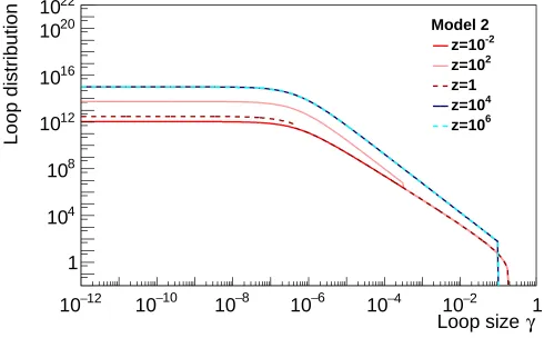
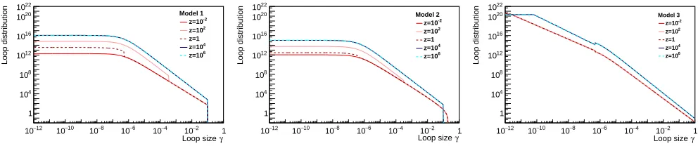
The loop distributionF(1) _{is plotted in Fig. 1 for} dif-ferent redshift values and fixingGµ at 10−8_{. A} discon-tinuity, visible for low redshift values, results from the radiation-matter transition which is modeled by Heavi-side functions. For t < teq, the loop distribution is

en-tirely determined by Eq. 3 and is time independent.

B. ModelM = 2: large loop Nambu-Goto distribution of Blanco-Pillado et al.

Rather than postulating that all loops are formed with a given sizeαtat timetas in model 1, the loop production function can be determined from numerical simulations. This approach was taken in [33], determining the rate of production of loops of size ℓ and momentum ~p at time

t. Armed with this information, n(ℓ, t) is determined analytically as in model 1 with the additional assumption

that the momentum dependence of the loop production function is weak so that it can be integrated out.

In the radiation era, the scaling distribution reads

F_rad(2)(γ) = 0.18 (γ+γd)5/2

Θ(0.1−γ), (8) where the superscript (2) stands for model 2. In the matter era, analogously to above, there are two contri-butions. The loops left over from the radiation era can be deduced from above, whereas loops formed in the matter era have distribution

Fmat(2),b(γ, t) =

0.27−0.45γ0.31 (γ+γd)2

Θ(0.18−γ)Θ(γ−β(t)),

(9) whereβ(t) is given in Eq. (5) withα= 0.1.

The loop distribution of model 2 is plotted in Fig. 1.

Notice that in the radiation era, the distributions in mod-els 1 and 2 take the same functional form, though their normalisation differs by a factor of order 10. In the mat-ter era, the functional form is slightly different and the normalisation is smaller by a factor of order 2. The au-thors of [33] attribute this reduction in the number of loops to two effects: (i) only about 10% of the power is radiated into large loops – indeed, most of it is lost di-rectly into smaller loops which radiate away very quickly; (ii) most of the energy leaving the network goes into loop kinetic energy which is lost to redshifting.

C. Model M= 3: large loop Nambu-Goto distribution of Ringeval et al.

This analytical model was presented in [34], and is based in part on the numerical simulations of [35].

As opposed to model 2, here the (different) numerical simulation is not used to determine the loop production function at timet, but rather the distribution of non-self intersecting loops at timet. The analytical modeling also differs from that of model 2 in that an extra ingredient is added: not only do loops emit GWs — which decreases their length ℓ — but this GW emission back-reacts on the loops. Back-reaction smooths out the loops on the smallest scales (in particular any kinks), thus hindering the formation of smaller loops [43, 49]. Hence, the distri-butions of models 2 and 3 differ for the smallest loops.

Physically, therefore, the model of [34] contains a fur-ther length scale γc, the so-called “gravitational back-reaction scale”, with

γc< γd,

where γd is the gravitational decay scale introduced above. Following the numerical simulation of [35],

γc= Υ(Gµ)1+2χ where Υ∼10 and χ= 1−P/2, (10) with

P = 1.41₋+00..0807

_mat, P = 1.60+0₋₀._.21₁₅

The resulting distribution of loops is given in [34].

In this paper, we work with the asymptotic expressions given in section 2.4 of [34], valid in the scaling regime (t≫tini). Hence the contribution of those loops formed

in the radiation era, but which persist into the matter era, are neglected. The loop distribution has three distinct regimes with different power-law behaviours, depending on whether the loops are smaller than γc (γ ≤ γc); of

intermediate length (γc ≤ γ ≤ γd); or larger than γd (that is γd ≤γ ≤γmax). Hereγmax = 1/(1−ν) is the largest allowed (horizon-sized) loop, in units of cosmic time, where the power-law time evolution of the scale factor of the universe,a∼tν_{, is}

ν = 2 3

_mat

, ν= 1 2 _rad . (12)

Hence,γmax= 2, orγmax= 3, depending on whether we are in the radiation-dominated or matter-dominated era, respectively. More explicitly,

•For loops with length scale large compared toγd: F(3)(γd≪γ < γmax)≃ C

(γ+γd)P+1

. (13)

•For loops with length scale in the rangeγc< γ≪γd: F(3)_(γ

c < γ≪γd)≃

C(3ν−2χ−1) 2−2χ

1

γd 1

γP . (14) • For loops with length scale smaller thanγc the distri-bution isγ independent:

F(3)_(γ≪γ

c≪γd)≃

C(3ν−2χ−1) 2−2χ

1 γP c 1 γd . (15)

Here,C is given by

C=C0(1−ν)3−P (16) where

C0 = 0.09−+00..0303

_mat, C0 = 0.21+0−0..1312

_rad. (17)

In the case of large loops (Eq. 13), C normalizes the distribution. In the radiation era whereν= 1/2,

C∼0.08 (radiation)

(a factor of about 20 smaller than model 1), and in the matter era whereν = 2/3,

C∼0.016 (matter) (a factor of about 30 smaller than model 1).

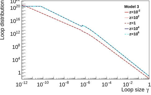
The three loop regimes are well-visible when plotting the loop distribution: see Fig. 1. Regarding the GW signal, the most significant difference between model 3 and the two previous models is in the very small loop regime (γ ≪ γc). Comparing Eq. 15 with Eq. 4 and

Eq. 8, for models 3, 1 and 2 respectively, in the radiation era, we find

F(3) F(1,2)

γ≪γc

∝(Gµ)−0.74 , (18)

where the proportionality constant is 2.5×10−2_{for model} 1 and approximately ten times larger for model 2. For a typical value of Gµ = 10−8_{, and relative to model 1,} there are∼2×104_{more very small loops in the radiation} era in model 3. As we will see in Sec. III, such a high number of small loops in model 3 will have important consequences in the rate of GW events we can detect and on the amplitude of the stochastic gravitational wave background.

III. CONSTRAINING COSMIC STRINGS

MODELS WITH GW DATA

A. Gravitational waves from cosmic strings

GW bursts are emitted by both cusps and kinks on cosmic string loops, the frequency-domain waveform of which was calculated in [44, 45, 50]:

h(ℓ, z, f) =Aq(ℓ, z)f−qΘ(fh−f)Θ(f−fℓ), (19)

whereq= 4/3 for cusps,q= 5/3 for kinks, andAq(ℓ, z)

is the signal amplitude produced by a cusp/kink propa-gating on a loop of sizeℓat redshiftz. This waveform is linearily polarized and is only valid if the beaming angle

θm(ℓ, z, f)≡(g2f(1 +z)ℓ)−1/3<1. (20) Here g2 is an ignorance factor assumed to be 1 in this work (see [32]). In order to detect the GW, the angle subtended by the line of sight and the cusp/kink on a loop of typical invariant lengthℓ at redshift z, must be smaller than θm. This condition then determines the

high-frequency cutoff fh in Eq. 19. The low-frequency

cutofffℓ — though in principle determined by the kink

amplitude, or by the size of the feature that produces the cusp — is in practice given by the lower end of the GW detector’s sensitive band. The amplitudeAq(ℓ, z) is

given by [44]

Aq(ℓ, z) =g1

Gµℓ2−q

(1 +z)q−1_r(z) , (21) where the proper distance to the source is given by

r(z) =H0−1ϕr(z). Here,H0is the Hubble parameter to-day andϕr(z) is determined in terms of the cosmological

12

−

10 ₁₀−10 ₁₀−8 ₁₀−6 ₁₀−4 ₁₀−2 ₁

γ Loop size 1 4 10 8 10 12 10 16 10 20 10 22 10 Loop distribution Model 1 -2 z=10 2 z=10 z=1 4 z=10 6 z=10 12 −

10 ₁₀−10 ₁₀−8 ₁₀−6 ₁₀−4 ₁₀−2 ₁

γ Loop size 1 4 10 8 10 12 10 16 10 20 10 22 10 Loop distribution Model 2 -2 z=10 2 z=10 z=1 4 z=10 6 z=10 12 −

10 ₁₀−10 ₁₀−8 ₁₀−6 ₁₀−4 ₁₀−2 ₁

γ Loop size 1 4 10 8 10 12 10 16 10 20 10 22 10 Loop distribution Model 3 -2 z=10 2 z=10 z=1 4 z=10 6 z=10

FIG. 1: Loop size distributions predicted by three models: M = 1,2,3. For each model, the loop distribution,

F(γ, t(z)), is plotted for different redshift values and fixingGµat 10−8_.

variables out ofℓ,zandAq. Similarly, we will use Eq. 19

to substituteAq for the strain amplitudeh.

For a given loop distribution modelM, in the following we use the GW burst rate derived in [32] and recalled in Appx. B:

d2_R(M)

q

dzdh (h, z, f) =

2NqH0−3ϕV(z)

(2−q)(1 +z)ht4_(z) ×F(M)

_ℓ(hfq_{, z)}

t(z) , t(z)

×∆q(hfq, z, f). (22)

The first two lines on the right-hand side give the num-ber of cusp/kink features per unit space-time volume on loops of size ℓ, where Nq is the number of cusps/kinks

per oscillation period T = ℓ/2 of the loop. In this pa-per, the number of cusps/kinks per loop oscillation is set to 1 although some models [51] suggest that this num-ber can be much larger than one. Cosmic time is given by t(z) = ϕt(z)/H0 and the proper volume element is

dV(z) =H0−3ϕV(z)dzwhere ϕt(z) andϕV(z) are given

in Appx. A. Finally ∆q, which is fully derived in Appx.B,

is the fraction of GW events of amplitudeAq that are

ob-servable at frequencyf and redshiftz.

B. Gravitational-wave bursts

We searched the Advanced LIGO O1 data (2015-2016) [30] for individual bursts of GWs from cusps and kinks. The search for cusp signals was previously con-ducted using initial LIGO and Virgo data and no signal was found [52].

For this paper, we use the same analysis pipeline to search for both cusp and kink signals. We perform a Wiener-filter analysis to identify events matching the waveform predicted by the theory [44, 45, 50] and given in Eq. 19. GW events are detected by matching the data to a bank of waveforms parameterized by the high-frequency cutoff fh, with 30 Hz< fh <4096 Hz. Then

resulting events detected at Hanford and at LIGO-Livingston are set in time coincidence to reject detector noise artifacts mimicking cosmic string signals. Finally, a

multivariate likelihood ratio [53] is computed to rank co-incident events and infer probability to be signal or noise. The analysis method is described in [52]. In this paper we only report on the results obtained from the analysis of new O1 LIGO data.

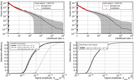
The upper plots in Fig. 2 present the final event rate as a function of the likelihood ratio Λ for the cusp and kink search. The rate of accidental coincident events be-tween the two detectors (background) is estimated by performing the analysis over 6000 time-shifted LIGO-Livingston data sets. This background data set virtually offers 2.5×1010 _{s (∼790.7 years) of double-coincidence} time. For both cusps and kinks, the candidate ranking values are compatible with the expected background dis-tribution, so no signal was found. The highest-ranked event is measured with Λh≃232 for cusps and Λh≃611

for kinks. These events were scrutinized and were found to belong to a known category of noise transients called “blips” described in [54], matching very well the wave-form of cusp and kink signals.

The sensitivity to cusp and kink GW events is esti-mated experimentally by injecting simulated signals of known amplitudeAq in the data. We measure the

detec-tion efficiencyeq(Aq) as the fraction of simulated signals

recovered with Λ > Λh, which is associated to a false

alarm rate of 1/Tobs = 2.40×10−7 Hz. The detection efficiencies are displayed in the bottom plots in Fig. 2. The sensitivity curve of the 2005-2010 LIGO-Virgo cusp search is also plotted, and should be compared with the O1 LIGO sensitivity measured for an equivalent false-alarm rate of 1.85×10−8_{Hz [52]. The sensitivity to} cos-mic string signals is improved by a factor 10. This gain is explained by the significant sensitivity improvement at low frequencies of Advanced detectors [30].

modelM :

R(M)

q (Gµ, p) = Z +∞

0

dAq eq(Aq) (23)

× Z +∞

0

dzd

2_R(M)

q

dzdAq

(Aq, z, f∗;Gµ, p)(24),

where the predicted rate is given by Eq. 22 with the change of variables Aq = hf−q. The frequency f∗ =

30 Hz is the lowest high-frequency cutoff used in the search template bank as it provides the maximum angle between the line of sight and the cusp/kink on the loop. The parameter space of modelM, (Gµ, p), is scanned and excluded at a 95% level when R(qM) exceeds2.996/Tobs

which is the rate expected from a random Poisson process over an observation timeTobs. The resulting constraints are shown in Fig. 6 and will be discussed in Sec IV.

C. Stochastic gravitational-wave background

Cosmic string networks also generate a stochastic back-ground of GWs, which is measured using the energy den-sity

ΩGW(f) =

f ρc

dρGW

df , (25)

where dρGW is the energy density of GWs in the

fre-quency range f to f +df and ρc is the critical energy

density of the Universe. Following the method outlined in [56], the GW energy density is given by:

Ω(GWM)(f;Gµ, p) =

4π2

3H2 0

f3 Z h∗

0

dh h2

×

Z +∞

0

dzd

2_R(M)

dzdh (h, z, f;Gµ, p),

(26)

where the spectrum is computed for a specific choice of free parametersGµandp, and the maximum strain am-plitudeh∗_{is defined below. This equation gives the}

con-tribution to the stochastic background from the super-position of unresolved signals from cosmic string cusps and kinks, and we shall determine the total GW energy density due to cosmic strings is by summing the two. Note that this calculationunderestimatesthe stochastic background since it only includes the high-frequency tribution from kinks and cusps. The low-frequency con-tribution from the smooth part of loops may be impor-tant, and has been discussed in [57–60]. Neglecting this contribution, conservative constraints will be derived.

To compute the integrals in Eq. 26 we adopt the numerical method described in Appx. B. As observed in [50], the integration over the strain amplitude is per-formed up to h∗ _{to exclude the individually resolvable} powerful and rare bursts. The maximum strain ampli-tudeh∗ _{determined by solving the equation}

Z +∞ h∗

dh

Z +∞

0

dzd

2_R(M)

dzdh (h, z, f) =f. (27)

This encodes the fact that when the burst rate is larger thanf, individual bursts are not resolved.

The total energy density in gravitational waves pro-duced by cosmic strings will be composed of overlapping signals (h < h∗_{) and non-overlapping signals, namely} bursts (h > h∗_{). The LIGO-Virgo stochastic search} pipeline will detect both types of signals. This has been demonstrated for a stochastic background produced by binary neutron stars, whose signals overlap, and binary black holes, whose signals will arrive in a non-overlapping fashion [61, 62]. In this present cosmic string study this effect is negligible: the predicted GW energy density, Ω(_GWM), does not grow significantly (and Fig. 3, top, does not change noticeably) whenh∗_→+∞.

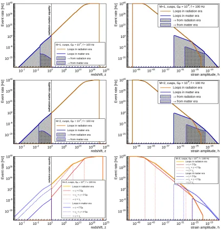
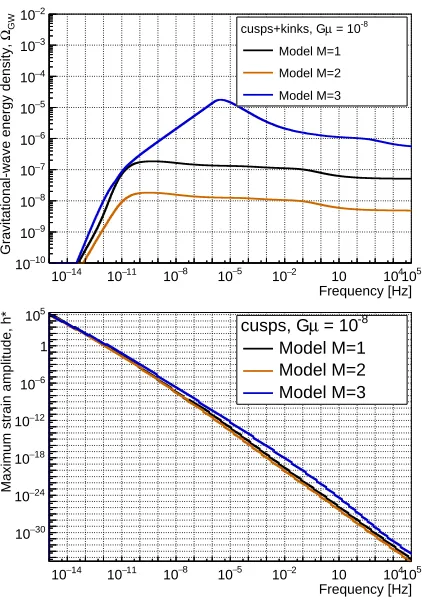
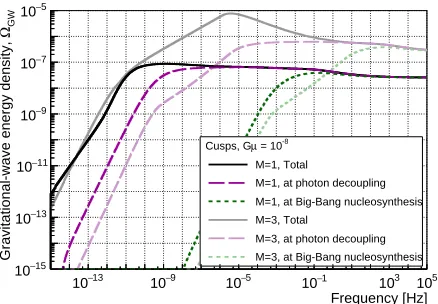
Fig. 3 (top) shows the spectra for the three models un-der consiun-deration, adding both the cusp and the kink con-tributions and assumingGµ= 10−8_{. Model 2 spectrum} is about 10 times weaker than the spectrum of model 1 over most of the frequency range. As shown in Fig. 4 (top), the spectra are dominated by the contribution of loops in the radiation era over most of the frequency range, including the frequencies accessible to LIGO and Virgo detectors (10-1000 Hz). The difference in normal-izations of the loop distributions in the radiation era in the two models, discussed in Sec. II, is therefore the cause for the difference in spectral amplitudes. Note also that at low frequencies (∼10−9 _{Hz), at which pulsar timing} observations are made, the matter era loops contribute the most.

Fig. 3 (top) also shows that the spectrum for model 3 has a significantly higher amplitude than those of models 1 and 2. Fig. 4 shows that this spectrum is dominated by the contribution of small loops which, as discussed in Sec. II, are much more numerous in model 3.

Fig. 3 (bottom) shows the maximum value for the strain amplitude to consider in the integration,h∗ _{as a} function of the frequency. At LIGO-Virgo frequencies (10-1000 Hz) the spectrum originates from GWs with strain amplitudes below∼10−28_.

The energy density spectra predicted by the mod-els can be compared with several observational results. First, searches for the stochastic GW background using LIGO and Virgo detectors have been performed, using the initial generation detectors (science run S6, 2009-2010) [63] and the first observation run (O1, 2015-2016) of the advanced detectors [31]. Both searches reported frequency-dependent upper limits on the energy density in GWs. To translate these upper limits into constraints on cosmic string parameters, we define the following like-lihood function:

lnL(Gµ, p)∝X i

−Y(fi)−ΩGW(M)(fi;Gµ, p) 2

σ2_(f

i)

, (28)

whereY(fi) andσ(fi) are the measurement and the

as-sociated uncertainty of the GW energy density in the frequency binfi, and Ω

(M)

GW(fi;Gµ, p) is the energy

1 10 ₁₀2 3

10 ₁₀4 5

10 Λ Likelihood ratio 11 − 10 10 − 10 9 − 10 8 − 10 7 − 10 6 − 10 5 − 10 4 − 10

Event rate [Hz]

Cusp search - LIGO O1 Background Candidates

1 10 ₁₀2 3

10 ₁₀4 5

10 Λ Likelihood ratio 11 − 10 10 − 10 9 − 10 8 − 10 7 − 10 6 − 10 5 − 10 4 − 10

Event rate [Hz]

Kink search - LIGO O1 Background Candidates

22 −

10 ₁₀−21 ₁₀−20 ₁₀−19 ₁₀−18

]

-1/3

[s

cusps

Signal amplitude, A 0 0.1 0.2 0.3 0.4 0.5 0.6 0.7 0.8 0.9 1 Detection efficiency

Sensitivity to cusp signals Hz

-7

10

×

LIGO O1, FAR=2.40 Hz

-8

10

×

LIGO O1, FAR=1.85 Hz

-8

10

×

LIGO 2005-2010, FAR=1.85

21 −

10 10−20 10−19 10−18 ₁₀−17

]

-2/3

[s

kinks

Signal amplitude, A 0 0.1 0.2 0.3 0.4 0.5 0.6 0.7 0.8 0.9 1 Detection efficiency

Sensitivity to kink signals

Hz

-7

10 × LIGO O1, FAR=2.40

FIG. 2: In the upper plots, the red points show the measured cumulative cusp (left-hand plot) and kink (right-hand plot) GW burst rate (usingTobs as normalization) as a function of the likelihood ratio Λ. The black line shows the expected background of the search with the±1σstatistical error represented by the hatched area. In both cases, the

highest-ranked event (Λh≃232 and Λh≃611) is consistent with the background. The lower plots show the

sensitivity of the search as a function of the cusp/kink signal amplitude. This is measured by the fraction of simulated cusp/kink events recovered with Λ>Λh. The sensitivity to cusp signals is also measured for a false-alarm

rate (FAR) of 1.85×10−6 _{Hz to be compared with the sensitivity of the previous LIGO-Virgo burst search [52]} (dashed lines).

frequency bin fi and for some set of model

parame-ters Gµ and p. We evaluate the likelihood function across the parameter space (Gµ, p) and compute the

95%confidence contours for the initial LIGO-Virgo (S6, 41.5 < f < 169 Hz) [63] and for the most recent Ad-vanced LIGO (O1, 20< f <86 Hz) [31] stochastic back-ground measurements (assuming Bayesian formalism and flat priors in the log parameter space). Since a stochas-tic background of GWs has not been detected yet, these contours define the excluded regions of the parameter space. We also compute the projected design sensitivity for the Advanced LIGO and Advanced Virgo detectors, using Eq. 28 withY(fi) = 0 and with the projectedσ(fi)

for the detector network [64].

Another limit can be computed based on the Pulsar Timing Array (PTA) measurements of the pulse arrival times of millisecond pulsars [29]. This measurement pro-duces a limit on the energy density at nanohertz fre-quencies — specifically, at 95% confidence ΩPTA

GW(f = 2.8×10−9 _Hz)<2.3×10−10_{. We directly compare the} spectra predicted by our models (at 2.8×10−9_{Hz) to} this constraint.

Finally, indirect limits on the total (integrated over frequency) energy density in GWs can be placed based

on the Big-Bang Nucleosynthesis (BBN) and Cosmic Mi-crowave Background (CMB) observations. The BBN model and observations of the abundances of the light-est nuclei can be used to constrain the effective num-ber of relativistic degrees of freedom at the time of the BBN, Neff. Under the assumption that only photons and standard light neutrinos contribute to the radia-tion energy density, Neff is equal to the effective num-ber of neutrinos, corrected for the residual heating of the neutrino fluid due to electron-positron annihilation:

Neff ≃3.046 [65]. Any deviation from this value can be attributed to extra relativistic radiation, including poten-tially GWs due to cosmic string kinks and cusps gener-ated prior to BBN. We therefore use the 95% confidence upper limit Neff −3.046 < 1.4, obtained by comparing the BBN model and the abundances of deuterium and 4_{He [27], which translates into the following limit on the} total energy density in GWs:

ΩBBN

GW (Gµ, p) =

Z 10

10

Hz

10−10

Hz

14 −

10 ₁₀−11 −8

10 10−5 ₁₀−2 _{10 10}4 5

10 Frequency [Hz] 10 − 10 9 − 10 8 − 10 7 − 10 6 − 10 5 − 10 4 − 10 3 − 10 2 − 10 GW Ω

Gravitational-wave energy density,

-8 = 10 µ cusps+kinks, G Model M=1 Model M=2 Model M=3 14 −

10 10−11 10−8 10−5 10−2 10 104105

Frequency [Hz] 30 − 10 24 − 10 18 − 10 12 − 10 6 − 10 1 5 10

Maximum strain amplitude, h*

-8 = 10 µ cusps, G Model M=1 Model M=2 Model M=3

FIG. 3: Top: GW energy density, Ω(GWM)(f), from cusps and kinks predicted by the three loop distribution models. The string tensionGµhas been fixed to 10−8_.

Bottom: maximum strain amplitudeh∗ _{used for the} integration in Eq.26.

BBN [60]. In this calculation we only consider kinks and cusps generated before BBN, which implies limiting the redshift integral in Eq. 26 toz >5.5×109_.

Similarly, presence of GWs at the time of photon decoupling could alter the observed CMB and Baryon Acoustic Oscillation spectra. We apply a similar proce-dure as in the BBN case, integrating over redshifts before the photon decoupling (z >1089) and over all frequencies above 10−15 _{Hz (horizon size at the time of decoupling)} to compute the total energy density of GWs at the time of decoupling. We then compare this quantity to the pos-terior distribution obtained in [28] to compute the 95%

confidence contours:

ΩCMBGW (Gµ, p) =

Z 1010 Hz

10−15 _Hz

dfΩ(GWM)(f;Gµ, p)<3.7×10−6, (30) For reference, Fig. 5 shows the energy density spectra for models 1 and 3 usingGµ= 10−8_{. As expected, the} contribution from the matter era loops is suppressed at the time of the BBN or of photon decoupling, resulting in the suppression of the spectra at low frequencies. To have negligible systematic errors associated to the numerical integration, we compute Eq. 29 and Eq. 30 using 200 and

13 −

10 10−9 10−5 ₁₀−1 3

10 105

Frequency [Hz] 12 − 10 11 − 10 10 − 10 9 − 10 8 − 10 7 − 10 6 − 10 5 − 10 4 − 10 GW Ω

Gravitational-wave energy density,

-8

= 10

µ

M=1, cusps, G Total

Loops in radiation era Loops in matter era

from radiation era

→

from matter era

→

13 −

10 10−9 10−5 10−1 103 105

Frequency [Hz] 10 − 10 9 − 10 8 − 10 7 − 10 6 − 10 5 − 10 4 − 10 3 − 10 GW Ω

Gravitational-wave energy density,

-8

= 10 µ M=3, cusps, G

Total

Loops in radiation era µ G Γ > γ → µ G Γ < γ < c γ → c γ < γ →

Loops in matter era µ G Γ > γ → µ G Γ < γ < c γ → c γ < γ →

FIG. 4: Top: GW energy density, Ω(GWM)(f), from cusps for model 1. We have separated the contributions from loops in the radiation (z >3366) and matter (z <3366)

eras. Additionally, for loops in the matter era, we have separated the effect of loops produced in the matter era

from the ones produced in the radiation era (Eq. 3, Eq. 4 and Eq. 6). Bottom: GW energy density, Ω(GWM)(f), from cusps for model 3. The effect of the three

loop size regimes is shown (Eq. 13, Eq. 14 and Eq. 15) for the matter and radiation eras.

250 logarithmically-spaced frequency bins respectively. Fig. 6 shows the excluded regions in the parameter spaces of the three models considered here, based on the stochastic observational constraints discussed above.

IV. DISCUSSION

The constraints on the cosmic string tensionGµ and intercommutation probabilityp are shown in Fig. 6 for the three loop models under consideration: M = 1 [8, 32] (top-left), M = 2 [33] (top-right) and M = 3 [34] (bottom-left). We recall that these three models were developed forp= 1 and, as explained earlier, for smaller intercommutation probability, we used a 1/pdependence for the loop distribution.

The bounds resulting from the burst search performed on O1 data are the least constraining. For model 3 and