1193.pdf

ABSTRACT

JAMES WORK MOORE. Operational Evaluation of Pilot GAC Filter Adsorbers (Under the Direction of DR. FRANCIS A. DIGIANO)

Granular activated carbon (GAC) filter-adsorbers are becoming widely used in the United States for control of taste and odor and synthetic organic compounds (SOCs). While filter-adsorbers are

relatively inexpensive to install, especially as retrofits to

existing filter beds, their limited empty bed contact times (EBCTs) and frequent backwashing may hamper control of organics.

A pilot plant consisting of three filter-adsorbers was installed at the Franklin WTP in Charlotte, N.C. Although the

focus of this investigation was on the microbial quality of the product water, other data were collected to assess the operational characteristics of of GAC as a filter and an adsorber of natural organic matter (NOM).

The GAC filter-adsorbers reduced turbidity as least as well as

the full-scale dual media filters at application rates of 2, 4, and

6 gpm/ft^ and backwash frequencies of one and two days. Similarly,

headloss accumulations in the filter-adsorbers were comparable to that in the full-scale dual media filters. The filter-adsorbers did not effectively remove TOC, as 50% breakthrough was observed in

less than 1 month for the lowest application rate in current

practice (2 gpm/ft^) . This poor performance was attributed to mass

gpm/ft^, but was observed to be no more than 0.5 mg/L. Some

TABLE OF CONTENTS

Page

1. INTRODUCTION...1

2 . BACKGROUND...3

3. METHODS AND MATERIALS

3 .1 Treatment Plant Description... 7

3 .2 Pilot Plant Description...9

3 . 3 Pilot Plant Operation...11

3.3.1 Pilot Plant Runs...13

3.3.1.1 Run One...14

3.3.1.2 Run Two...15

3.3.2 Procedure for Backwashing...15

3.4 Measurement of Turbidity...17

3 . 5 Measurement of Headloss...17

3.6 Measurement of Total Organic Carbon...18

3.7 Measurement of Trihalomethane Formation Potential...18

3 . 8 Determination of GAC Adsorption Isotherm...19

4. RESULTS AND DISCUSSION

4 .1 Turbidity Removal...20

4.1.1 Raw and Settled Water Turbidity...20

4.1.2 Effect of Appplication Rate on Removal...23

4.1.3 Effect of Backwashing on Removal...25

4.1.4 Conclusions...25

4 . 2 Headloss Accumulation...27

4.2.1 Effect of Application Rate...27

4.2.2 Effect of Backwashing...31

4.2.3 Conclusions...3 4

4 . 3 TOC Removal...3 5

4.3.1 TOC Removal— Run One...35

4.3.2 Approach to Steady State Removal— Run One...40

4.3.3 TOC Removal— Run Two...43

4.3.4 Approach to Steady State Removal— Run Two...45

4.3.5 TOC Profiles in Filter-adsorbers...48

4.3.6 TOC Adsorption Modelling...51

4.4 Removal of Trihalomethane Formation Potential...56

5 . CONCLUSIONS AND RECOMMENDATIONS...63

6 . REFERENCES...67

LIST OF TABLES

3 .1 Pilot Plant Media Characteristics...13

3 . 2 Pilot Plant Feedwater Characteristics...13

3 . 3 Pilot Plant Runs...14

3 . 4 Instructions for Backwashing of Filter-Adsorbers...16

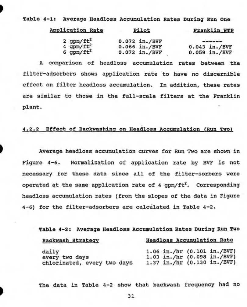
4 .1 Average Headloss Accumulation Rates During Run One...29

4 . 2 Average Headloss Accumulation Rates During Run Two...31

4.3 T-test Analyses on Significance of Run One Steady-State TOC Removal...41

LIST OF FIGURES

Ifege

3 .1 Franklin WTP Flow Diagram...8

3 . 2 Pilot Filter-adsorber Diagram...10

3 . 3 Schematic of Pilot Plant...12

4 .1 Franklin WTP Turbidities...22

4 . 2 Run One Filtered Water Turbidities...24

4 . 3 Run Two Filtered Water Turbidities...26

4 . 4 Run One Average Headloss Accumulations...28

4 . 5 Run One Average Headloss Accumulations...3 0 4 . 6 Run Two Average Headloss Accumulations...32

4 . 7 Run One TOC Breakthrough Curves...3 6 4 .8 Run One TOC Breakthrough Curves...37

4 . 9 Run One TOC Breakthrough Curves...39

4 .10 Run One TOC Removal vs. TOC Applied...42

4 .11 Run Two TOC Breakthrough Curves...44

4.12 Run Two TOC Breakthrough Curves...46

4.13 Run Two TOC Removal vs. TOC Applied...47

4 .14 Run One TOC Profiles— Day 107...49

4 .15 Run One TOC Removal vs • EBCT— Day 107...50

4.16 Run Two TOC Profiles— Day 21...52

4 .17 Calgon Filtrasorb 300 8x30 GAC Isotherm...54

4 .18 HSDM Predicted TOC Breakthrough...57

4.19 Comparison of Predictive Models to Run 2 TOC Breakthrough..58

4.20 Run One THMFP Removal...59

ACKNOWLEDGEMENTS

This report is the end result of contributions made by several caring individuals who should not go unnoticed.

I would like to take this opportunity to thank Professor Fran DiGiano for his counsel and input into this research. I would also like to thank Drs. Mike Aitken and Don Francisco for their

contributions to this report, and Professor Phil Singer for his academic guidance throughout my education at UNC-CH. Additional thanks goes to David Chang for his invaluable assistance and

patience in the laboratory.

Many thanks and congratulations goes to the staff of the Franklin WTP for their input into the installation and operation of the pilot plant. I would also like to thank Nathan Cobb for his

many contributions to the set-up of the pilot plant and for making

the project more enjoyable to work on.

My deepest gratitiude to my family for their love and support and to all of my friends for making my stay in Chapel Hill such a wonderful experience. Finally, I would like to thank Kim for her

love, respect, and support.

This investigation was conducted as part of a research program

supported by the American Water Works Association Research

CHAPTER 1. INTRODUCTION

Granular activated carbon (GAC) filter-adsorbers are becoming widely used for control of taste and odor and synthetic organic compounds (SOCs). While filter-adsorbers are relatively inexpensive to install, especially as retrofits to existing filter beds, their limited empty bed contact times (EBCTs) and frequent backwashing may hamper control of organics.

The water utilities industry in the United States is interested in the problems associated with retrofitting beds with GAC. The American Water Works Association Research Foundation (AWWARF) sponsored a pilot plant study of GAC filter-adsorbers at the Franklin Water Treatment Plant in Charlotte, North Carolina. The primary focus of this investigation was on the microbial quality of product water and generation of carbon fines.

The scope of work for this project was divided into the following three aspects:

1. General operations of filter-adsorbers including total organic carbon (TOC) removal, turbidity removal, and

headless accumulation.

2. Microbial activity on GAC.

3. Generation of carbon fines.

Previous reports by Cobb (1990) and Mallon (1991) discussed

Proper operation of the pilot plant is a necessary first step in the overall study. Additionally, this report analyzes the breakthrough and steady state removal of NOM. Limited adsorptive capacity renders GAC filter-sorbers economically infeasible as a method of reduction for most NOM and SOCs. However, microbial biodegradation may allow steady state removal over significant periods of time. This would allow utilities to implement GAC

filter-adsorbers to the new MCLs as set forth by amendments to the SDWA. The results presented in this paper both support and complement the scope of the AWWARF project.

The specific objectives of the studies described in this report

were:

1. Construct AWWARF filter-adsorber pilot plant at the Franklin WTP in Charlotte, North Carolina and develop operational procedure.

2. Evaluate performance of pilot filter-adsorbers as a

filter.

CHAPTER 2. BACKGROUND

Granular activated carbon (GAC) is currently being used in over 150 water treatment plants in the United States (Schuliger, 1988). The primary use for GAC in water treatment is the removal of tastes and odors, which have been effectively removed with bed lives of 1-5 years (Graese et. al., 1987). In some cases, (e.g. Jefferson Parish, LA; Cincinnati, OH) GAC is employed to remove trihalomethane formation potential (THMFP). However, the short bed life for removal of these compounds is cost intensive, and thus

application is not very widespread.

Across Europe, GAC is placed in post-filter adsorbers for

removal of THMFP or other specific SOCs. In the United States, GAC is commonly used in place of granular media in conventional rapid filters (GAC filter-adsorbers) for both turbidity and organics removal (Graese et. al., 1987). Experience has shown GAC to be as effective as sand for turbidity removal (Hyde et. al., 1987).

The question of whether filter-adsorbers can be used to meet future maximum contaminant levels (MCLs) for specific compounds is

important because of lower capital cost compared to post-filter

adsorbers. Although effective for removal of taste and odor, use

of filter-adsorbers for THMFP and other weakly-adsorbed compounds is limited. One reason for this is the limited EBCTs available due

to restraints imposed by existing filter structures in sand-replacement filters. Shortened EBCTs require more rapid

regeneration of GAC, resulting in higher costs.

backwash. Solids loading on filter-adsorbers requires more frequent backwashing, which causes a redistribution of particles

within the bed, elongation of the mass transfer zone (MTZ) , and

faster breakthrough of the contaminant(s) (Cairo et. al., 1979). It is not yet fully understood if post-filter adsorbers are advantageous to filter-adsorbers with respect to backwash frequency. Experience shows that post-filter adsorbers must be backwashed eventually, although certainly not as often as

filter-adsorbers. Research has shown no noticeable difference in

performance of GAC backwashed every day versus GAC backwashed every

thirty days (Weisner et. al., 1987). '

Design and operation of GAC processes are influenced by their placement in the treatment scheme. Two important considerations for design of filter-adsorbers are media size and EBCT. Media

selection for filter-adsorbers must accommodate both filtration and

adsorption requirements. GAC media characteristics influence headless development, filter run length, backwash requirements, and filtered water quality. A survey of several treatment plants in the United States shows filter-adsorbers to average 15 to 3 0 inches of 12x40 mesh (0.55-0.65 mm) or 8x30 mesh GAC (0.80-0.90) over two to twelve inches of sand (Graese et. al., 1987). These sizes of GAC provide the proper combination of effective size and uniformity coefficient to promote adsorption while allowing for longer filter

runs and better cleaning.

1986). In addition, as EBCT increases, the ratio of MTZ to EBCT decreases, and the specific volume of water treated increases (Hand et. al., 1989). A survey of filter-adsorbers in used show an average EBCT of 8.6 minutes with a range of 3.2 to 24.8 minutes. These filter-adsorbers produced an average effluent turbidity of 0.3 NTU with an average filter run length of 55 hours when fed at

an application rate of 1 to 4 gpm/ft^ (Graese et. al., 1987).

Much of current research is focused on microbial activity in GAC beds. Bioactivity on GAC is encouraged in several Western European countries, e.g. Germany, France, and the Netherlands. Microbes existing on GAC biodegrade organic compounds leading to increased steady state removal and longer bed life. Research has shown biodegradation to remove 8.5% - 16% of influent TOC (Maloney, 1984). This removal may be further enhanced by pre-ozonation

(Maloney et. al., 1986).

In U.S. water treatment plants, however, practice is often to impair or preclude development of biological activity by pre¬ chlorination, rigorous scouring of filter media, and frequent backwashing (Bouwer, 1988). This is largely due to concern over the possible release of microbially-populated carbon fines into the distribution system. Populated GAC filter fines have been found in drinking water from numerous properly operated treatment facilities (McFeters, 1987). Bacteria on GAC has been found to be resistant to 2.0 mg/L chlorine for up to one hour of exposure (McFeters, 1987) . This trade-off of enhanced organic removal versus the

CHAPTER 3. METHODS AND MATERIALS

3.1 Treatment Plant Description

The 72 MGD Walter M. Franklin Water Treatment Plant (WTP), built in 1958 and upgraded in 1967, 1981, and 1990, currently produces three-fourths of the water used by customers in the Charlotte Mecklenburg Utility District (CMUD). A schematic of the Franklin WTP process train is shown in Figure 3-1. The water is treated by coagulation, flocculation, sedimentation, filtration,

and disinfection.

The raw water is supplied from Mountain Island Lake which is fed from Lake Norman, an impoundment on the Catawba River. Water from Mountain Island Lake is pumped to a 250 million gallon reservoir located next to the plant for temporary storage prior to treatment. Characteristics of the water are given below:

Plant flowrate: 35-40 MGD

Turbidity: 3-25 NTU, avg= 8 NTU Threshold Odor Number: 7-9, avg= 8

Alkalinity: 10-15 mg/L as calcium carbonate

---—^ A

PAC CL 2 ALUM

I /

I MOUNTAIN

1 1 1

RAPID MIX FLOCCULATION SEDIMENTATION FILTRATION

\ ISLAND \ "

j LAKE \

FL —ͨ

v^.--^

CL2---

LIME-DISTRIBUTION

itig/L) are added to the filtered water prior to release into the distribution system.

3.2 Pilot Plant Description

The pilot plant was located in the basement of the filter building at the Franklin WTP. Settled water from the Franklin WTP

was used as feed for the pilot plant, eliminating the need for simulation of coagulation, flocculation, and sedimentation

processes.

The pilot plant consisted of three polyvinyl chloride filter

housings having a height of 13 0 in. and a diameter of 4 in. A

diagram of a typical pilot filter-adsorber is shown in Figure 3-2.

These contained 3 0 in. of GAC over 12 in. of sand. A valved feed

line near the top of the housing delivered water from the Franklin WTP sedimentation basin. Also near the top of the housing were the filter overflow and backwash exit lines, both connected to the drain. The location of the filter-adsorber overflow allowed for 6

ft of water on top of the media and 9.5 ft of total available head

through the media. The columns were equipped with Camp nozzle underdrains that connected to three valved lines for filtered water

effluent, backwash feed, and air scour. Sample ports were located at GAC depths of 2, 15, and 3 0 in. to allow for collection of water

and media. In addition, other sample ports throughout the media

FEED FROM

MANIFOLD

-H-<o

o

CM

V

WATER

GAC

SAND

MANOMETER TUBES FOR HEADLOSS MEASUREMENT

-H-n

OVERFLOW BW EXIT TO DRAIN TO DRAIN

WATER/GAC

SAMPUNG PORTS

CAMP NOZZLE

BW AIR SCOUR FILTER FEED EFF

measurement.

The flow diagram for the pilot plant is given in Figure 3-3.

Water was taken from a position in sedimentation basin at the

Franklin Plant that was approximately 3 ft below the surface and directly below the overflow weir. The water was gravity-fed to the pilot plant feed manifold, which consisted of ball valves to

distribute flow to the filters. Water from the manifold flowed in

excess to the top of the filters. Variable-speed centrifugal pumps, connected to the filter underdrains, controlled the flow through the filters. Any excess water from the manifold drained through the filter overflows. Feed water and filtered water samples were collected at taps located at the manifold and pump

suction, respectively.

Filtered water was pumped into 55 gallon clearwells. Overflow

taps at the top of the clear wells drained excess flow while keeping the wells full at all times. The clearwells served as

reservoirs for backwash water. Pilot plant valving allowed for the variable-speed centrifugal pumps to also be used as backwash pumps. During backwashing, filtered water was pumped from the clearwells, back through the filters and out the backwash drain at the top of the filter. Backwashing was augmented with air scour.

3.3 Pilot Plant Operation

OVERFLOW TO WASTE 1 MANIFOLD CLEAR WELL #3 COMPRESSED __i n AIR PUMP #3 BACKWASH UNE CLEAR WELL #2 T

1

I

rtzi FILTER

Franklin WTP sand and 3 0 in. of fresh 8x3 0 GAC (Calgon Filtrasorb

300) . The specific characteristics of the media are listed in

Table 3-1.

Table 3-1: Pilot Plant Media Characteristics

Media Depth Effective Size Uniformity Coefficient GAC 30 in. 0.8-0.9 mm 1.9-2.4

sand 12 in. 0.5 mm

The characteristics of 8x3 0 GAC closely resemble anthracite; this GAC is widely used in filter-adsorbers (Graese et. al., 1987). The sand provided an extra barrier against turbidty breakthrough. The filters were backwashed with filtered plant water several times after charging to assure initial carbon fine removal and bed stratification. Feedwater supplied to the pilot plant for Runs

One and Two was Franklin Plant settled water. Characteristics of

the feedwater for both runs are given below in Table 3-2.

Table 3-2: Pilot Plant Feedwater Characteristics

Parameter Run 1 Run 2 pH 6.1-7.0 6.0-6.8

Average Turbidity, NTU 1.1 0.7

Average Color 9 9

Alkalinity, mg/L as CaC03 15 15

3.3.1 Pilot Plant Runs

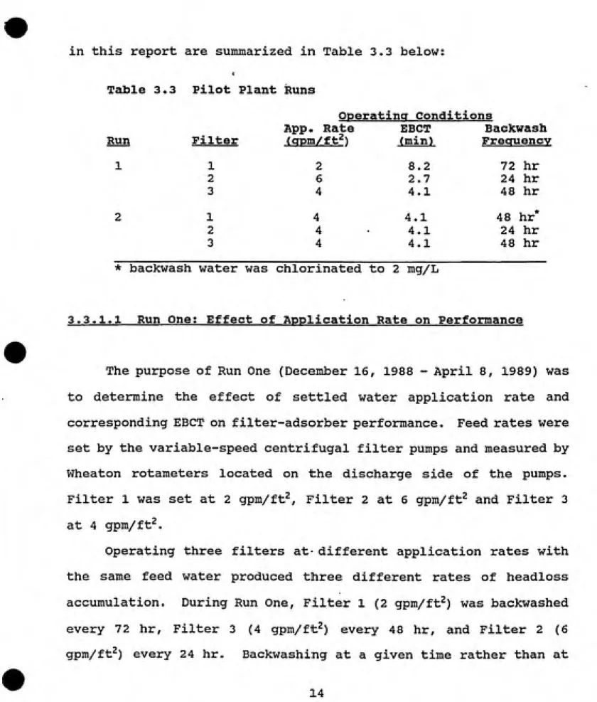
in this report are summarized in Table 3.3 below:

Table 3.3 Pilot Plant Runs

Operating Conditions

App. Rate EBCT Backwash

Run Filter (acm/ft^^ (min) _Frequency

1 1 2 8.2 72 hr

2 6 2.7 24 hr

3 4 4.1 48 hr

2 1 4 4.1 48 hr*

2 4 4.1 24 hr

3 4 4.1 48 hr

* backwash water was chlorinated to 2 mg/L

3.3.1.1 Run One: Effect of Application Rate on Performance

The purpose of Run One (December 16, 1988 - April 8, 1989) was

to determine the effect of settled water application rate and corresponding EBCT on filter-adsorber performance. Feed rates were set by the variable-speed centrifugal filter pumps and measured by

Wheaton rotameters located on the discharge side of the pumps.

Filter 1 was set at 2 gpm/ft^. Filter 2 at 6 gpm/ft^ and Filter 3

at 4 gpm/ft^.

Operating three filters at different application rates with the same feed water produced three different rates of headless

accumulation. During Run One, Filter 1 (2 gpm/ft^) was backwashed

every 72 hr. Filter 3 (4 gpm/ft^) every 48 hr, and Filter 2 (6

gpm/ft^) every 24 hr. Backwashing at a given time rather than at

a designated headloss assured adeguate plant staff availability in case of breakdown and minimized operator oversight. The standard backwash procedure used for all filter-adsorbers during Run One is

discussed in Section 3.3.2 of this report.

Operators monitored the pilot plant every four hours, checking and recording application rates, and filter effluent turbidities, and filter headlosses. Turbidity and headloss measurements are

discussed later in Section 3.4 and 3.5 of this report.

3.3.1.2 Run Two; Effect of Backwashinq Strategy on Performance

The purpose of Run Two (May 17-August 7, 1989) was to

determine the effect of backwash strategy on filter-adsorber performance. During Run Two, all filters were run at an

application rate of 4 GPM/ft^. Filters 1 and 3 were backwashed

every 24 hr, and Filter 2 every 48 hr. Filter 1 washwater was chlorinated to 2 mg/L by adding approximately 40 mL of chlorine bleach to Clearwell 1 prior to backwashing. Actual backwashing procedure and pilot plant monitoring were continued as in Run One.

3.3.2 Procedure for Backwashinq of Filter-Adsorber

The standard backwashing procedure used during Runs One and

Two was developed in accordance with recommendations from the

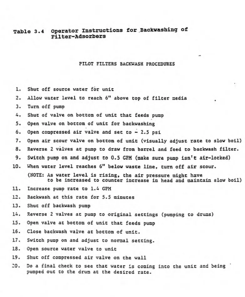
Table 3.4 operator Instructions for Backwashing of

Filter-Adsorbers

PILOT FILTERS BACKWASH PROCEDURES

1. Shut off source water for unit

2. Allow water level to reach 6" above top of filter media

3. Turn off pump

4. Shut of valve on bottom of unit that feeds pump 5. Open valve on bottom of unit for backwashing 6. Open compressed air valve and set co - 2.5 psi

7. Open air scour valve on bottom of unit (visually adjust rate to slow boil)

8. Reverse 2 valves at pump to draw from barrel and feed to backwash filter.

9. Switch pump on and adjust to 0.5 GPM (make sure pump isn't air-locked)

10. When water level reaches 6" below waste line, turn off air scour. (NOTE: As water level is rising, the air pressure might have

to be increased to counter increase in head and maintain slow boil)

11. Increase pump rate to 1.4 GPM

12. Backwash at this rate for 5.5 minutes 13. Shut off backwash pump

14. Reverse 2 valves at pump to original settings (pumping to drums)

15. Open valve at bottom of unit that feeds pump

16. Close backwash valve at bottom of unit.

17. Switch pump on and adjust to normal setting.

18. Open source water valve to unit

19. Shut off compressed air valve on the wall

20. Do a final check to see chat water is coming into the unit and being

procedure in the form of operator's instructions. The initial

backwash rate was 5 gpm/ft^ and included air scour. After

approximately 2 minutes, the air scour was ceased, and the backwash

rate was increased to 14 gpm/ft^ for 5.5 minutes.

3.4 Measurement of Turbidity

Hach Low-Range Process Turbidimeters sampled water from the discharge lines of the filter pumps. Turbidity measurements were recorded every four hours by the plant operators during routine inspection. The turbidimeters were calibrated according to manufacturer's specifications by the Franklin plant instrument staff prior to the start of each run.

3.5 Measurment of Headloss

Filter headlosses were measured by tygon manometer tubes that were inserted into ports located along the depth of the

filters. The tubes were attached to a board which was marked-off in 0.2 5 ft increments. The total headloss across the filter was the difference in water levels of manometer tubes connected to

ports located at points in the filter freeboard and underdrain. Operators recorded total headloss every four hours during routine

3.6 Measurement of Total Organic Carbon

Total organic carbon (TOC) samples were analyzed with an 0. I.

Corporation Model 7 00 TOC Analyzer. Samples introduced into the 01

700 were automatically acidified with 5% phosphoric acid, purged to

remove inorganic carbon, and analyzed to measure inorganic carbon.

After the purging step, sodium persulfate (100 g/L) was introduced

to the sample in a 100°C reactor to oxidize the organics to carbon

dioxide. The carbon dixoide was subsequently purged to an IR

detector and measured against a linear KHP calibration to yield TOC

(actually non-purgeable organic carbon). The specifications for

the linear assumption and + 2% of full scale error of

repeatability for sample concentrations greater than 0.002 mg/L

(Harrington, 1987).

TOC samples were collected daily in 40 ml septum vials. The

samples were dosed with concentrated nitric acid to inhibit

biological activity, refrigerated, and analyzed within two weeks of

collection.

3.7 Measurement of Trihalomethane Formation Potential (THMFP)

Samples analyzed for THMFP were buffered with a phosphate

buffer solution and chlorinated to 2 0 mg/L with a stock solution of

sodium hypochlorite. After a five day incubation period in the

dark, the samples were analyzed for remaining chlorine residual,

and THMs were extracted using a liquid/liquid technique. The

solvent used was n-pentane with carbon tetrachloride as an internal

standard. After extraction, THMs were chromatagraphed on SP-1000

using a GC equipped with a '^^Ni electron capture detector. For a

more detailed description of THMFP analytical procedures, refer to

Reckhow (1984).

3.8 Determination of GAG Adsorption Isotherm

The equilibrium adsorption of TOC in plant settled water was

determined using the bottle point method as described by Randtke

and Snoeyink (1983). GAC (Filtrasorb 300) was prepared by washing

with distilled-deionized water, drying at 110°C and grinding to 200

X 325 U.S. Standard mesh size. After preparation, different

dosages of activated carbon were added to 16 bottles, each

containing 100 mL of settled water from the Franklin WTP with a

known TOC concentration of 1.47 mg/L. Activated carbon doses

ranged from 2 to 2 40 mg/L; one bottle contained no activated

carbon. Phosphate buffer (3 mg/L) and sodium azide (5 mg/L) were

added to the sample bottles to maintain pH and inhibit biological

degradation of TOC, respectively. The bottles were then placed on

a tumbler and equilibrated for 7 days at room temperature.

After equilibration, the samples were filtered with 0.45 um

been pre-soaked to remove any residual TOC. The TOC of the samples

was measured after filtration.

CHAPTER 4. RESULTS AND DISCUSSION

4.1 Turbidity Removal

4.1.1 Raw and Settled Water Turbidity During Pilot Plant Studies

Results of turbidity measurements made during this study are

presented in the form of frequency plots in Figures 4-1.

Inspection of these data shows that 95% of the time the raw water

turbidity during Run One was less than 4.8 NTU and 50% of the time

the NTU was less than 2.7. During Run Two, 95% of the time the raw

water turbidities were less than 9.2 NTU and 50% of the time less

than 6.7 NTU.

The higher raw water turbidity found in Run Two than Run One

was attributed to seasonal lake dynamics. Changes in temperature

cause lakes to turn over during the spring and fall. Associated

with these turnovers is increased turbidity as murky water near the

bottom of the lake is cycled to the surface. Run Two occurred May

17-August 7 and included water from the spring turnover. Run One,

on the other hand, occurred December 16-April 8, between the fall

and spring turnovers. The difference in raw water turbidities

Figure 4.1 Franklin WTP Turbidities

10

8

ͣ

a n

3

^RAW1 -4-RAW 2 -^ SETTLED 1 ^ SETTLED 2

100

4.1.2 Effect of Application Rate on Turbidity Removal (Run One)

Filtered water turbidity data from Run One is presented in Figure

to all three filters, it was assumed that the feed water was of the

same turbidity. The data in Figure 4-2 show that the same product

water turbidity was obtained regardless of application rate.

Although 4 gpm/ft^ is widely considered standard practice for a

filter application rate, Lykins and Adams (1989) give several

examples of comparable filter performance at application rates to

6 gpm/ft^. Further, Graese et. al. (1987) reports successful

turbidity removal by 8x3 0 GAC and sand filters at filter

application rates ranging from 1 to 3.5 gpm/ft^. In addition, it

would appear that the GAC pilot filter-sorbers were more effective

at turbidity removal than the Franklin dual media sand-anthracite

filters: 90% of filtered water turbidity values from the pilot

filter-adsorbers were less than 0.02 NTU as compared to 90% of the

values from the Franklin dual media filters being 0.10 NTU. While

GAC has been shown to be better than anthracite for turbidity

removal due to increased surface angularity (Hyde, 1987), the

inaccuracy of the turbidimeters at turbidities this low (less than

0.1 NTU) prevent drawing a definite conclusion.

Figure 4.2 Run One Filtered Water Turbidities

0.24

0.2

0.16

=3

I-^ 0.12

ͣ

u

0.08

0.04

2 GPM/SQFT 6 GPM/SQFT

4- 4 GPM/SQFT

-^- FRANKLIN

100

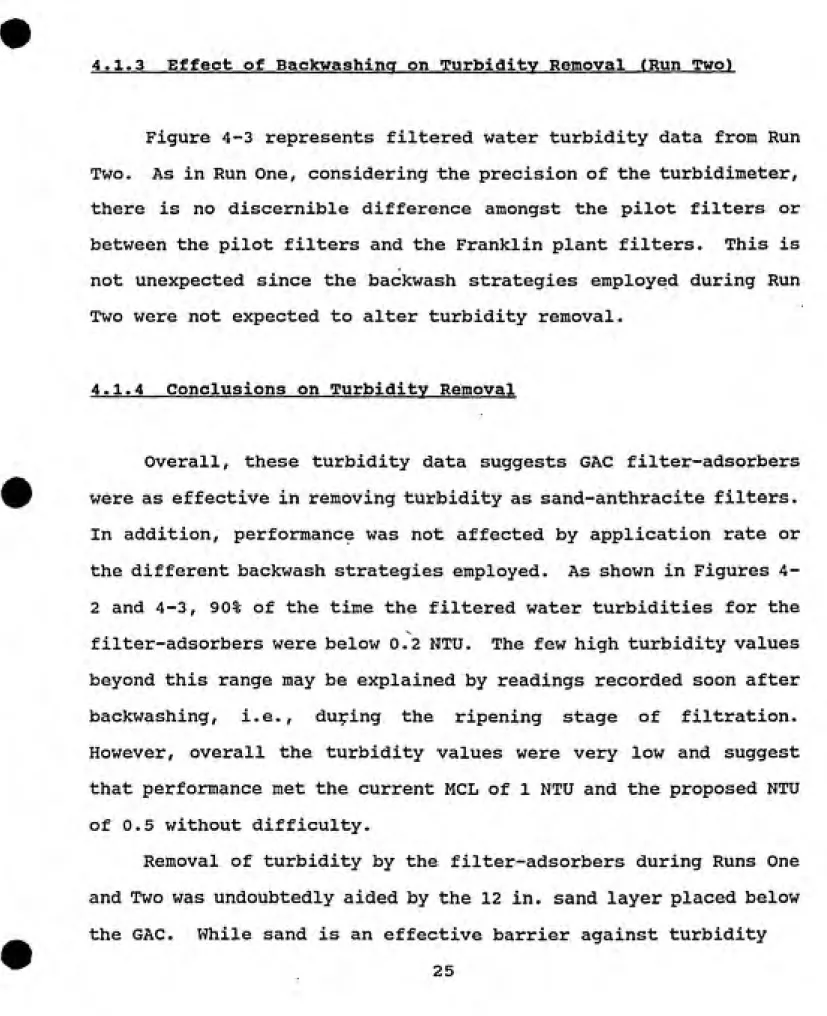
4.1.3 Effect of Backwashinq on Turbidity Removal (Run Two)

Figure 4-3 represents filtered water turbidity data from Run

Two. As in Run One, considering the precision of the turbidimeter,

there is no discernible difference amongst the pilot filters or

between the pilot filters and the Franklin plant filters. This is

not unexpected since the backwash strategies employed during Run

Two were not expected to alter turbidity removal.

4.1.4 Conclusions on Turbidity Removal

Overall, these turbidity data suggests GAC filter-adsorbers

were as effective in removing turbidity as sand-anthracite filters.

In addition, performance was not affected by application rate or

the different backwash strategies employed. As shown in Figures

4-2 and 4-3, 90% of the time the filtered water turbidities for the

filter-adsorbers were below 0.2 NTU. The few high turbidity values

beyond this range may be explained by readings recorded soon after

backwashing, i.e., during the ripening stage of filtration.

However, overall the turbidity values were very low and suggest

that performance met the current MCL of 1 NTU and the proposed NTU

of 0.5 without difficulty.

Removal of turbidity by the filter-adsorbers during Runs One

and Two was undoubtedly aided by the 12 in. sand layer placed below

Figure 4.3 Run Two Filtered Water Turbidities

0.24

0.16

0

BWCL2 BW1 BW2 FRANKLIN

20 40 60 80 100

breakthrough, it also reduces the adsorptive capacity of the

filter-adsorber by taking up filter-box volume that would otherwise

be occupied by additional GAC. THe occupation of filter-box volume

by sand can be even more problematic for existing filter boxes that

are relatively shallow. The Coliform Rule, as part of amendments

to the Safe Drinking Water Act, sets a maximum level for turbidity

at 0.5 NTU. The filtered water turbidities were much lower than

this goal, and suggests less sand could have been used. Further

investigations should address the proper depth of sand layer to

maintain compliance with the Coliform Rule while maximizing the

adsorption capacity of the filter-adsorber.

4.2 Headless Accumulation

Each filter run generated a series of headless data. Headloss

readings were then organized with respect of time into each filter

run. All of these individual filter runs were averaged over the

entire pilot run (two to three months of data) in order to generate

representative curves for headloss accumulation. Included with the

curves are confidence intervals with a coefficient (1 - a) =0.95.

Both filter run time and volume of water filtered to a given filter

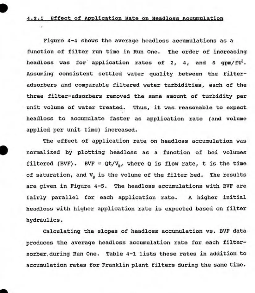
Figure 4.4 Run One Average Headloss Accumulations

2.5

CD

(0 m

o T3

CO <D X

0

— 2 QPM/SF -1-4 QPM/SF -^ 6 QPM/SF

20 40 60 80

4.2.1 Effect of Application Rate on Headloss Acctimulation

Figure 4-4 shows the average headloss accumulations as a

function of filter run time in Run One. The order of increasing

headloss was for application rates of 2, 4, and 6 gpm/ft^.

Assuming consistent settled water quality between the

filter-adsorbers and comparable filtered water turbidities, each of the

three filter-adsorbers removed the same amount of turbidity per

unit volume of water treated. Thus, it was reasonable to expect

headloss to accumulate faster as application rate (and volume

applied per unit time) increased.

The effect of application rate on headloss accumulation was

normalized by plotting headloss as a function of bed volumes

filtered (BVF) . BVF = Qt/Vg, where Q is flow rate, t is the time

of saturation, and Vg is the volume of the filter bed. The results

are given in Figure 4-5. The headloss accumulations with BVF are

fairly parallel for each application rate. A higher initial

headloss with higher application rate is expected based on filter

hydraulics.

Calculating the slopes of headloss accumulation vs. BVF data

produces the average headloss accumulation rate for each

filter-sorber, during Run One. Table 4-1 lists these rates in addition to

Figure 4.5 Run One Average Headloss Accumulations

2.6

eo"

(0

o

d)

1.5

0.5

0

— 2 QPM/SF -4- 4 QPM/SF -^ 6 QPM/SF

100 200 300

Bed Volumes Filtered (BVF)

Table 4-1: Average Headloss Accumulation Rates During Run One

Application Rate Pilot Franklin WTP

2 gpm/ft^ 0.072 in./BVF

4 gpm/ft^ 0.066 in./BVF 0.043 in./BVF

6 gpm/ft^ 0.072 in./BVF 0.059 in./BVF

A comparison of headloss accumulation rates between the

filter-adsorbers shows application rate to have no discernible

effect on filter headloss accumulation. In addition, these rates

are similar to those in the full-scale filters at the Franklin

plant.

4.2.2 Effect of Backwashinq on Headloss Accumulation (Run Two)

- Average headloss accumulation curves for Run Two are shown in

Figure 4-6. Normalization of application rate by BVF is not

necessary for these data since all of the filter-sorbers were

operated at the same application rate of 4 gpm/ft^. Corresponding

headloss accumulation rates (from the slopes of the data in Figure

4-6) for the filter-adsorbers are calculated in Table 4-2.

Table 4-2: Average Headloss Accximulation Rates During Run Two

Backwash Strategy Headloss Accumulation Rate

daily 1.06 in./hr (0.101 in./BVF)

every two days 1.03 in./hr (0.098 in./BVF)

chlorinated, every two days 1.37 in./hr (0.13 0 in./BVF)

t

Figure 4.6 Run Two Average Headloss Accumulations

BWCL2

0 10 20 30

Filter Run Time, hours

effect on headless accumulation rate. However, the filter-adsorber

backwashed with chlorinated water exhibited a much higher rate.

This is not easily explained. It is possible that chlorine had a

brittling effect on the GAC; however, at 2 mg/L, only 0.076 grams

of mass chlorine were added to this filter-adsorber during

backwashing. This is small compared to the 5.2 grams of chlorine

received by all of the filter-adsorbers from the feed water during

every filter run.

Over time, the shape and/or size of the media could have been

changed due to numerous backwashings. However, filter runs during

the first 5 days of Run Two averaged headless accumulations of 1.32

in./hr while filter runs during the last 5 days average 1.3 5

in./hr. It is evident that time was not a factor. This would also

rule out any biological explanation considering the

filter-adsorbers would become more populated with time.

Another possible explanation is operator error in measuring

headless. A comparison of headloss data between the two runs shows

larger confidence intervals in Run Two. This suggests the data

were not as consistent throughout this run. It is possible the

manometer tubes became fouled with activated carbon dust and more

difficult to read over time. Assessing the confidence intervals in

Figure 4.6, it is difficult to determine if the difference in the

slopes of the curves is real or the result of error in measurement.

Expressing headloss accumulation rates as in./BVF allows

comparison of results from Runs One and Two. The operation of the

filter-adsorber backwashed every other day during Run Two is

identical to the operation of the filter-adsorber with an

application rate of 4 gpm/ft^ during Run One. While similar

headloss accumulation rates would have been expected, that in Run

Two was much higher. One possible explanation is a change in

settled water quality between the two, pilot-plant runs. Section

3.1 of this report described differences in raw and settled water

turbidity in the two pilot runs. Raw water turbidity was higher in

Run Two than in Run One but settled water turbidity remained about

the same. Nevertheless, the higher raw water turbidity meant an

increase in floe in the sedimentation basins. The intake for the

pilot plant was located approximately 3 ft. below the surface of

the sedimentation basins. Thus, the settled water turbidity

measured by plant personnel is not necessarily the actual turbidity

entering the pilot plant. It is possible that the increased amount

of floe in the sedimentation basins resulted in a higher

concentration of floe (and thus higher turbidity) to the pilot

filter-adsorbers during Run Two. This would explain the higher

headloss accumulation rates.

4.2.3 Conclusions on Headloss Accumulation

Overall, the performance of the filter-adsorbers was

comparable to conventional filters over a range of application

rates and backwash conditions. The explanation for increased rate

of headless in the chlorinated-backwash filter-adsorber remains

unclear. Perhaps the additional floe in the feedwater to the pilot

plant during Run Two was not evenly distributed by the manifold,

and this particular filter received a heavier load. Alternatively,

errors in reading the manometer tubes could have occurred. As

noted in Section 3.1, sand used in the filter-adsorbers may not be

necessary to prevent turbidity breakthrough. Eliminating the sand

layer may lessen the rate of headless accumulation.

4.3 TOC Removal

4.3.1 TOC Removal— Run One

The effect of application rate on TOC adsorption was

investigated in Run One. As application rate increased, the

adsorbate loading rate (mass/time) increases and the EBCT of the

filter-adsorber decreases. According to the simple eguilibrium

adsorption model, loading rate increases and the time to reach

exhaustion of adsorbent capacity should decrease. As EBCT

decreased, the ratio of the MTZ to EBCT increases thereby causing

the MTZ to comprise a larger portion of the length of the

filter-adsorber. If the MTZ is large (due to slow mass transfer

characteristics) , as is the case for NOM, more adsorbate escapes

into the product water and less of the total adsorptive capacity is

Figure 4.7 Run One TOG Breakthrough Gurves

CJ)

E

d

o

0

D

n

if +

0

+

-f. _m

+ 4- +

^^

^ 2 GPM/SF 4- 4 GPM/SF

ͤ

6 GPM/SF

25 50 75 100 125

Figure 4.8 Run One TOG Breakthrough Curves

1.2

o

O

o

0.2 f

0

+ +

-4-+ _| 1 U E "

+

4-i

+

' 2 GPM/SQFT -f 4 QPM/SQFT ---6 QPM/SQFT

utilized.

Figure 4-7 presents TOC breakthrough data from Run One.

Samples for Day 1 were collected immediately after start-up of the

filter-adsorbers. Presence of TOC in these samples suggest either

a non-adsorbable fraction of TOC or severe mass transfer

limitations caused by insubstantial EBCT.

A comparison of fractional TOC breakthrough curves is

presented in Figure 4-8 by normalizing the product water TOC data

by the average feed TOC. The general trend (although the data show

considerable scatter) is for TOC breakthrough to occur later as

application rate decreased. For example, 50% breakthrough occurs

almost immediately for the application rate of 6 gpm/ft^, whereas

it occurs between Day 11 and Day 15 for 4 gpm/ft^ and between Day

22 and Day 28 for 2 gpm/ft^.

The effect of application rate on mass loading rate of TOC can

be normalized by plotting TOC breakthrough as a function of BVF

rather than time. As shown in Figure 4-9, it is difficult to

determine one common shape for the initial pattern of the

breakthrough. This suggests that the effect of mass loading rate

alone may not explain differences with application rate.

The effect of increasing the ratio of MTZ to EBCT as

application rate is increased can also be examined. The amount of

TOC adsorbed to some target TOC in the product water is calculated

for each adsorber by subtracting the area under the

filter-adsorber breakthrough curve (Figure 4-7) from the area under the

Figure 4.9 Run One TOG Breakthrough Curves

1.2

o

O o

rtlT

cP

0

0 10

^ 2 QPM SF n 4 QPM/SF

20 30 40 50

6 QPM/SF

60 70

feed water TOC curve. This area is calculated up to the time when 1 mg/L of TOC appears in the product water, or Days 9, 12, and 23

for the 6, 4, and 2 gpm/ft^ filter-adsorbers, respectively. Using

the trapezoidal rule for area calculations, TOC removed at each

application was 29 grams at 2 gpm/ft^, 24 grams at 4 gpm/ft^, and

16 grams at 6 gpm/ft^. The decrease in TOC removal with increasing

application rate suggests that the effect of MTZ/EBCT ratio is

important.

4.3.2 Approach to Steady State Removal— Run One

After adsorption capacity is exhausted, removal of adsorbate

can continue to be realized through biodegradation. Data shown

after Day 100 in Figure 4-8 suggest that steady state removal of

TOC may be occurring, though scatter in the data prevents drawing

a definite conclusion. T-tests analyses were performed to

determine at what level the differences between the average

feedwater TOC concentration after Day 100 (Up) and the average

filtered water TOC concentrations after Day 100 (Uj, u^, u^) were

statistically significant. Results from these analyses, summarized

in Table 4-3, show removal of TOC to be statistically significant

at a confidence level greater than 99% for application rates of 2

gpm/ft^ and 4 gpm/ft^. Removal for the application rate of 6

gpm/ft^ was shown to be at a much lower confidence level, as was

the difference between the 2 and 4 gpm/ft^ removals.

Table 4-3: T-test Analyses on Significance of Run One

Steady-State TOC Removal

Scunple

TOC mg/L

Mean,u Stdrd. Dev. Samples

Feed 2 GPM/ft^ 4 GPM/ft^ 6 GPM/ft^ 2.63 2.04 2.19 2.43 0.12 0.32 0.32 0.29 9 9 9 9 Null Hypothesis (^4 ^2) ^2) 0 0 0 0 T-value 5.23 3.90 1.93 1.00 p-value < 0.01 < 0.01

0.05 < p < 0.10 > 0.20

To further evaluate the attainment of TOC steady-state

removal, the mass of TOC removed for each filter-adsorber was

plotted with respect to mass of TOC applied in Figure 4.10. These

data were obtained by using the areas under feed and breakthrough

curves in Figure 4-7 as explained in Section 4.3.1.

During the initial stage of filter-adsorber operation, the

mass of TOC removed per mass of TOC applied (i.e., the slope of

Figure 4.10) is considerably larger than the later stage. Other

investigators (Maloney et. al., 1984) have interpreted the shift in

removal rate to an exhaustion of adsorption capacity and an

attainment of some constant removal rate due to biodegradation. If

adsorption alone were occurring, the rate of TOC removal would

Figure 4.10 Run One TOG Removal vs. TOG Applied

140

120

(0 100 E

m

>

O E

cc

o o

2 QPM/SF 4 QPM/SF ^K-6 QPM/SF

200.0 400.0 600.0 800.0

TOG Applied, grams

slowly decrease and the slope in Figure 4-10 would reach zero. Alternatively, biodegradation would lead to a steady-state removal, or constant slope. Although the data during the later stage of

filter-adsorber do not describe a perfectly linear relationship,

there is reasonable evidence for a steady state condition. The

steady- state removal is not clearly shown to increase with decreasing application rate as may be expected if a large EBCT was important for achieving biodegradation.

4.3.3 TOC Removal— Run Two /

Backwashing is known to redistribute media, even in beds with high uniformity coefficients. Redistribution of GAC in an

adsorption column results in elongation of the mass tranfer zone

and faster breakthrough of TOC (Hand et. al., 1989). Other researchers (Graese et. al. , 1987) also report decreases in time of

breakthrough due to backwashing. However, in another report, Wiesner et. al. (1987) concludes that while backwashing reduced the time of breakthrough, there was little difference in breakthrough of filter-adsorbers backwashed daily versus filter-adsorbers

backwashed monthly.

Figure 4-11 shows the feed TOC and the TOC breakthrough curves for three different backwash strategies used in Run Two. All three filter-adsorbers were operated at the same application rate (4

Figure 4.11 Run Two TOC Breakthrough Curves

SETTLED -f BWCI2 ^ BW1

ͤ

BW2

-f

to be the same if backwashing strategy had no effect. These suggest this to be true. A similar conclusion is reached from Figure 4-12, in which the breakthrough curves have been normalized by the average feed concentration of TOC. Thus, TOC breakthrough was not noticeably altered by increasing the backwash frequency by a factor of two (once every day compared to once every two days) nor by addition of chlorine to the backwash water.

4.3.4 Approach to Steady State Removal— Run 2

TOC removed during Run Two is plotted against TOC applied in

Figure 4-13. For comparison, the corresponding data for the

application rate of 4 gpm/ft^ from Run One (backwashing once every

two days) are also shown. While TOC removal rate was initially the same for all three filter-adsorbers in Run Two, the rate at later stages was measureably lower for the filter-adsorber backwashed with chlorine than those backwashed without chlorine. This could be an indication of less microbial activity in the bed. In earlier reported work at this pilot plant, Cobb (199 0) found that the

filter-adsorber backwashed with chlorine released statistically less heterotrophic plate count; this is also an indication of less microbial activity. All of the removal rates in Run Two were

higher than that in Run One (at the same application rate). The only difference between the two runs is temporal: Run One was

Figure 4.12 Run Two TOC Breakthrough Curves

o

O

o

*

m

ffi

BWCL2 + BW1 _ͤ BW2

20 40 60

Day of Run

Figure 4.13 Run Two TOC Removal vs. TOC Applied

150 S

k_ D)

>

O E

0) cc

o

O

h-BWCL2 ^ BW1 -^ BW2 -^ Run 1

100

conducted in late spring and summer. Both higher water temperature

and different TOC character could explain the higher removal rate toward the end of Run Two if biodegradation was the dominant effect. Alternative explanations are possible having to do with

changes in adsorbability of TOC but no conclusions are possible

because the adsorption isotherm was determined only once in this

study (during Run Two).

4.3.5 TOC Profiles in Filter-adsorbers

Water samples were withdrawn at various depths in the

filter-adsorbers on Day 107 of Run One and Day 21 of Run Two. The TOC

profile on Day 107 should correspond to that for steady-state removal. As indicated in Figure 4-14, TOC did not decrease very much with depth as may be expected if significant biodegradation was occurring. Also shown is the TOC concentration for Franklin WTP filtered water on Day 107 of Run One. This level indicates the full-scale dual media filters were not removing TOC. The

filter-adsorber TOC data can be plotted against EBCT at each depth for

each application rate as shown in Figure 4-15. Aside from the slight increase in TOC noted at the top of the filter-adsorbers,

the overall trend is of a decrease in TOC with an increase in EBCT.

This observation is consistent with previous findings in this chapter indicating adsorption and biodegradation to be dependent of EBCT. A simple linear removal rate of 0.06 mg/L/min EBCT was

Figure 4.14 Run One TOC Profile— Day 107

E

O

O

^ 2 GPM/SQFT EH 4 GPM/SQFT W 6 QPM/SQFT

m

I

I

FEED

I

I

I

I

I

^

I

I

i

15 28

1

I

i

Figure 4.15 Run One TOG Removal vs. EBCT— Day 107

E

d

o

0

Y = 2,79 - 0,0613 X

0 4 6

Empty Bed Contact Time, minutes

calculated from Figure 4-15. This rate becomes an important design

parameter to determine if adequate steady state removal of TOC is

possible in a filter-adsorber. As an example, an EBCT of 25 minutes would be required to realize 50% removal of 3 mg/L TOC.

In contrast to the TOC profile on Day 107, that on Day 21 of Run 2 should reveal the presence of an adsorption front because

adsorptive capacity had not yet been exhausted. The resulting TOC

profile given in Figure 4-16 shows that 50% of the TOC was removed

in the first 2 in. of GAC. TOC removal occurred to a much less

extent deeper in the bed. This suggests a long MTZ as is expected for natural organic matter. Moreover, TOC at the bottom of the

filter-adsorber is higher than the refractory concentration (0.2

mg/L) found in the adsorption isotherm (Figure 4.7). This is

consistent with the idea that the MTZ was not contained, and thus

the EBCT (4.1 min) was to short to provide the most effective

adsorption.

4.3.6 TOC Adsorption Modelling

Results from an isotherm performed on Franklin WTP settled water using pulverized Filtrasorb 300 are listed in Table 4.4. The fraction of non-adsorbable TOC can be estimated by noting the amount of TOC that remains at high dosages of activate carbon. The

values in the last 5 rows of Column 3 indicate this non-adsorbable

non-Figure 4.16 Run Two TOG Profiles— Day 21

E

d

o

0

[^^ CI2 EZ] BW2 ^ BW1

'<<>'

<^

1

m

m

^

FEED 2 15

Depth, inches GAG

28

1

Table 4.4 GAG Isotherm Data

d) (2) (3) (4) (5)

M Go Ge Gorr. Ge _q

(g/L) (mg/L) (mg/L) (mg/L) (mg/g)

\ 0:002;

0.020 1.47 0:79 o:6i? 34.0000 0.030 1.47 0.63 0.45 28.0000 0.035 1.47 0.49 0:31

_{i 28:ooob|}

0.040 1.47 0.50 0.32 24.25001 1 0.050 1.47 0.47 0:29 i 20:0000

0.060 1.47 0.38 0.2 18.1667

0;080 1.47 0:29 • o:riit; 14:7500 0.100 1.47 0.22 0.04 12.5000 0.120 1.47 0:19 0:01 10.6667

0.140 1.47 0.18 0

9.2143 1

8:06251

0.240 1.47 0.18 0

5:3750 1

Regression Output:

Constant 1.72670635

StdErrofYEst 0.09657122

R Squared 0.86605649

No. of Observations 12

Degrees of Freedom 10

X Coefficient(s) 0.560 = 1/n

Std Err of Coef. 0.070

t-calc 8.041

f

Figure 4.17 Calgon Filtrasorb 300 8X30 GAC Isotherm

100

D) E

0.1

adsorbable fraction, the data were fitted to a Freundlich isotherm

model: q = k C^''", where k = 53.29 and 1/n = 0.56. The correlation

of this fit was 0.87 and the calculated T-value was 8.04. Figure

4-17 is a plot of the corrected isotherm data along with the

A rough estimate of time for TOC breakthrough can be

calculated by assuming that adsorption is not rate limited using

the following equilibrium adsorption model:

tg = (k * C^i/" * W) / (Q * CJ

where,

tg = time of TOC breakthrough

k, 1/n = Freundlich parameters

C^ = settled water TOC concentration = 1.5 mg/L

W = mass of GAC in filter-sorber = 3 000 g Q = volumetric flowrate ,

This model uses the isotherm data and mass of GAC to calculate the

TOC adsorption capacity of the filter-adsorber, and then estimates

time of breakthrough using the amount of TOC applied daily. The

equilibrium adsorption model predicts complete breakthrough for

application rates of 2, 4, and 6 gpm/ft^ can be to occur at 139,

70, and 4 6 days, respectively. These are conservative estimates of

service time because mass transfer limitations cause some fraction

of sorbate to escape adsorption and appear in the product water

earlier than the equilibrium model predicts (JMM, 1985).

To account for some of the mass transfer limitations and gain

isotherm data corrected for non-adsorbable TOC and a volumetric

flowrate of 4 gpm/ft^, the HSDM model calculated an immediate TOC

breakthrough of 35%, 50% breakthrough in 42 days, and 95% breakthrough in 349 days. The entire predicted breakthrough curve is presented in Figure 4-18. The model calculations used for generating this breakthrough curve are presented in Appendix A. For a complete description of the simplified HSDM model, refer to

Hand et. al. (1984).

Equilibrium and HSDM model predictions are plotted with actual Run Two TOC breakthrough curves in Figure 4-19. The comparison of

the HSDM model and the actual data to the equilibrium model gives

an indication of the mass transfer limitations imposed by the restricted EBCT at the given application rates.

4.4 Removal of Trihalomethane Formation Potential

The removal of TOC by filter-adsorbers also implies removal of precursors of THMs. Thus, this study included measurements of

THMFP. Due to limited laboratory equipment availability, testing

during Run One was limited to three days during the last three

weeks of the run. However, these data are still useful for assessment of THMFP removal at steady state. In Run Two, THMFP

tests were conducted on five days throughout the entire length of

the run.

The THMFP of feed and product water on three days toward the

Figure 4.18 HSDM Predicted TOC Breakthrough

o

O O

•100 0 100 200 300 400 500 600 700

Figure 4.19 Comparison of Predictive Models to Run 2 TOC Breakthrough

0.8

o 0.6 O

O

0.4

0.2

0

Equilibrium

ͣͣ

"

_ͣͣ

: n

°

m ~

ͣ

D

„

^

ͤ

of «*

pW^^"^ HSDM

B

^SV^

ffi

-^^S-^

0+^

ͤ

:' "H-

9

B

1 1 1

^ BWCL2 + BW1 ͤ BW2

1 1

0 20 40 60

Day of Run

Figure 4.20 Run One THMFP Removal

100

80

C3) =3 CL

IE

60

40

20

0

FEED ^2 GPM/SQFT [MSI 4 QPM/SQFT ^ 6 QPM/SQFT

end of Run One are shown in Figure 4-20. The TOC breakthrough curves and adsorption model predictions (Section 4-3.5) imply that adsorption capacity was exhausted during this time period and any removal was most likely due to biodegradation. Data in Figure 4-2 0 reveals THMFP removal ranged from 5-4-2 0 ug/L with greater removals being realized at lower application rates (higher EBCTs). While these reductions may not be meaningful based on effluent goals anticipated from EPA, it is possible that further increases in EBCT could yield more THMFP removal. The data also suggest that THMFP removal, like TOC removal, had reached a steady state.

The THMFP data from Run Two are presented in Figure 4-21. Much greater THMFP removal was obtained on Days 3 and 9 than later in the run. However, some breakthrough of THMFP (10-20 ug/L) was noted. This implies that a fraction of NOM responsible for formation of THMs is not adsorbable. This is an important consideration for assessing the effectiveness of GAG for eliminating precursors to THM formation. Removal of 2 5-4 0 ug/L THMFP was still occurring approximately one month into Run Two. However, the THMFP had increased to 40 ug/L. The THMFP data from Day 72 suggest that feedwater concentration dropped preciptuously and that THMFP exceeded the feedwater concentration, possibly as a result of desorption. However, the corresponding feed TOC concentration on Day 72 was not appreciably lower than previous

(see Figure 4-11). This raises some concern about the accuracy of

the THMFP data (THMFP should roughly correlate to TOC) and suggests

Figure 4.21 Run Two THMFP Removal

too

=3

Q."

LL

FEED BW2 BWCL2

caution in interpreting desorption as an explanation for higher

THMFP in the product water from the feed water. Finally, no difference was found in THMFP removal with backwashing strategy, i.e., all three filter-adsorbers produced about the same THMFP. This is consistent with observations made on TOC removal in Section

4.3.3.

CHAPTER 5. CONCLUSION AND RECOMMENDATIONS

The GAG filter-adsorbers, consisting of 3 0 in. of 8x3 0 Filtrasorb 3 00 over 12 in. of sand, were shown to reduce turbidity at least as well as the full-scale dual media filters at application rates of 2, 4, and 6 gpm/ft^ and backwash frequencies

of one and two days.

Headless accumulation in the filter-adsorbers were comparable to that in the full-scale dual media filters. The rate of headless accumulation (with respect to bed volumes of water filtered) was about the same regardless of application rate. Similiarly, headless accumulation rate did not depend on backwash frequency

(once per day versus once every two days). However, headless

accumulation rate was about 3 0% higher when backwashing with chlorinated washwater; no explanation for a higher rate could be

found.

Overall, the pilot filter-adsorbers performed adequately as

filters. They produced water of acceptable turbidity without

excessive accumulation of headless over a range of practical application rates and backwash frequencies. The GAG used in this application (Filtrasorb 300) has a small effective size and large uniformity coefficient which facilitates longer filter runs and

penetration of turbidity.

The breakthrough of TOC occurred earlier as application rate increased. Using 50% TOC breakthrough for illustration, breakthrough was immediate at 6 gpm/ft^, at between Days 11 and 15 for 4 gpm/ft^, and between Days 22 and 28 for 2 gpm/ft^. The data

showed very little potential for control of TOC unless EBCT could

be extended greatly. Earlier breakthrough of TOC with higher

application rate is due to two effects: (1) higher sorbate loading rate and (2) shorter EBCT relative to MTZ. The latter effect was shown by measuring the amount of TOC adsorbed up to a selected TOC concentration in the product water (1 mg/L) . The mass of TOC adsorbed decreased as application rate increased. Steady state removal of TOC was found to be statistically significant (T-test)

at a confidence level greater than 99% for the application rates of

2 and 4 gpm/ft^. Nonetheless, the amount was only about 0.5 mg/L.

Steady-state removal at 6 GPM/ft^ was statistically insignificant at a much lower confidence level as was the difference between 2 and 4 GPM/ft^. The data suggested some small amount of removal was

due to biodegradation at steady state.

Backwash frequency and chlorination of backwash water had no

effect on the initial pattern of TOC breakthrough. However, backwashing with chlorinated washwater appeared to decrease steady

state removal. This could imply that chlorination limited

microbial activity to some extent. Steady-state removal of TOC was

greater in Run Two than Run One. One possible explanation is more

biodegradation in Run Two due to higher water temperature and/or

A depth profile of TOC in the filter-adsorbers during the

early stages of Run Two showed the presence of an adsorption zone.

However, profiles measured during the later stages of Run One

showed a more linear decrease in TOC with depth, as may be expected

if biodegradation was important. The steady-state removal rate was

calculated to be 0.06 mg TOC/L/min EBCT.

A small, steady-state removal of THMFP (5-2 0 ug/L) was

obtained in Run One, with removal increasing as application rate

decreased. More data were collected in Run Two covering the entire

time of filter-adsorber operation. These data showed a refractory

THMFP of 10-20 ug/L. Removal of THMFP was found to be 25-40 ug/L

up to five weeks into the run. Again the importance of these

numbers is dependent upon the new maximum contaminant levels.

Overall, data from this study suggest filter-adsorbers are not

an effective means for removal of TOC. Data showed 50%

breakthrough in less than 1 month for the lowest filter application

rate in current practice (2 gpm/ft^) . Bed lifes of this length

would require frequent regeneration or replacement of GAC, with the

resulting high maintenance costs negating the capital costs saved.

One technology not studied was ozonation of the settled water

prior to application. Ozone has been shown to oxidize NOM to forms

preozonation to increase microbial activity and lengthen bed life. The following recommendations are made for future studies on GAC

filter-adsorbers:

1. Vary the depth of sand below the GAC to determine minimum amount necessary to meet turbidity standards and give good overall performance while maximizing EBCT of GAC.

2. Determine if enough EBCT can be established to facilitate

adequate steady-state removal of NOM to control

disinfection byproducts.

3. Determine if preozonation enhances steady-state removal of

NOM by biodegradation in filter-adsorbers.

CHAPTER 6. REFERENCES

Bouwer, E.J. and P.B. Crowe. "Biological Processes in Drinking Water Treatment." Journal AWWA, 80:9:82 (Septeinber 1988).

Cairo, P.R. "The U.S. Experiences- Pilot Plant Testing of Activated Carbon Adsorption Systems." Journal AWWA,

71:11:60 (November 1979).

Cobb, N.C. "Microbial Acitivity on GAC Filter-Adsorbers," Masters

Technical Report, University of North Carolina at Chapel Hill,

1990.

Committee Report: "An Assessment of Microbial Activity on GAC."

Crittenden, J.C.; Luft, P. and D.W. Hand. "Prediction of Fixed-Bed Adsorber Removal of Organics in Unknown Mixtures." Journal Environmental Engineering, 113:3:486 (March 1987).

Graese, S.L.; Snoeyink, V.L. and R.G. Lee. "Granular Activated Carbon Filter-Adsorber Systems." Journal AWWA, 79:12:64

(December 1987).

Hand, D.W.; Crittenden, J.C.; Arora, H.; Miller, J.M. and B.W. Lykins, Jr. "Designing Fixed-Bed Adsorbers to Remove

Mixtures of Organics." Journal AWWA, 81:1:67 (January 1989).

Hand, D.W.; Crittenden, J.C. and W.E. Thacker. "Simplified Models

for Design of Fixed-Bed Adsorption Systems." Journal of Environmental Engineering, 110:2:440 (April 1984).

Harrington, G.W. "The Effects of Coagulation, Ozonation, and

James M. Montgomery, Consulting Engineers, Inc. Water Treatment

Principles and Design, Wiley, New York, 1985.

Hyde, R.A.; Hill, D.G.; Zebel, T.F. and T. Burke. "Replacing Sand with GAC in Rapid Gravity Filters." Journal AWWA, 79:12:26

(December 1987).

Lykins, Jr., B.W. and R.M. Clark. Granular Activated Carbon.

Lewis, Chelsea, 1989.

Mallon, K.S. "....GAC Filter-Adsorbers...," Masters Technical Report, University of North Carolina at Chapel Hill, 1991.

Maloney, S.W.; Bancroft, K.; Pipes, W.O. and I.H. Suffet.

"Bacterial TOC Removal on Sand and GAC." Journal Environmental

Engineering Division- ASCE, 110:3:519 (1984).

Maloney, S.W.; Suffet, I.H.; Bancroft, K. and H.M. Neukrug.

"Ozone-GAC Following Conventional Drinking Water Treatment." Journal

AWWA, 77:8:66 (August 1985).

McFeters, G.A.; Camper, A.K.; LeChevallier, M.W.; Broadaway, S.C.

and D.G. Davies. "Bacteria Attached to Activated Carbon in

Drinking Water," Environmental Research Brief, U.S. Environmental Protection Agency, June 1987.

Randtke,S. and V.L. Snoeyink. "Evaluating GAC Adsorptive Capacity."

Journal AWWA, 75:8:406 (August 1983).

Reckhow, D.A. "Organic Halide Formation and the Use of Pre-Ozonation and Alum Coagulation to Control Organic Halide Precursors," Ph.D. thesis. University of North Carolina at

Chapel Hill, 1984.

Standard Methods for the Examination of Water and Wastewater,

1980. AWWA, WPCF, and APHA, eds.

Weisner, M.R.; Rook, J.J. and F. Fiessinger. "Optimizing the

Placement of GAC Filtration Units." Journal AWWA, 79:12:39

(December 1987).