Cycle Time Enhancement by Simulated Annealing for a Practical Assembly
Line Balancing Problem
Mai Huong Dinh∗
Hanoi University of Science and Technology, Hanoi, Vietnam Hanoi University of Industry, Hanoi, Vietnam
E-mail: [email protected]
Viet Dung Nguyen∗, Van Long Truong, Phan Thuan Do∗, Thanh Thao Phan and Duc Nghia Nguyen Hanoi University of Science and Technology, Hanoi, Vietnam
E-mail: [email protected], [email protected],
{thuan.dophan, thao.phanthanh}@hust.edu.vn,in the memory of Professor Duc Nghia Nguyen
Keywords:assembly line balancing, simulated annealing, meta-heuristic
Received:March 15, 2020
In the garment industry, assembly line balancing is one of the most significant tasks. To make a product, a manufacturing technique called assembly line is utilized, where components are assembled and transferred from workstation to workstation until the final assembly is finished. Assembly line should always be as balanced as possible in order to maximize efficiency. Different types of assembly line balancing problems were introduced along with many proposed solutions. In this paper, we focus on an assembly line bal-ancing problem where the upper bound of the number of workers is given, tasks and workers have to be grouped into workstations so that the cycle time is minimized, the total number of workers is minimized and balance efficiency is maximized. With unfixed number of workstations and many other constraints, our problem is claimed to be novel. We propose three different approaches: exhaustive search, simulated annealing and simulated annealing with greedy. Computational results affirmed that our simulated anneal-ing algorithm performed extremely good in terms of both accuracy and runnanneal-ing time. From these positive outcomes, our algorithms clearly show their applicability potential in practice.
Povzetek: Problem uravnoteženja proizvodne poti je predstavljen odprto, brez omejitev npr. števila delavcev, zato je izviren. Avtorji testirajo veˇc algoritmov in predlagajo najboljšega.
1
Introduction
The assembly line consists of a set of workstations ar-ranged along a material transport system. Parts of the clothes are assembled on workstations, which are trans-ported from workstation to workstation in one direction until the final product is completed. Workers perform a number of tasks in each workstation to create the product. The assembly line rhythm, which is called the cycle time, is the average time for each workstation to complete its tasks before transferring the product’s subassembly to the next workstation. After that, the workstations receive new sub-assembles and repeat the assigned work.
In the fashion industry, patterns of clothing are ever-changing, each product has a set of tasks to assemble the details of clothes together. Each task has unique time to be performed on a specific type of machine or done man-ually. Among tasks there are precedence relationships, where some tasks must be performed before some other tasks to create a certain clothing product. Different prod-ucts will have different numbers of tasks and the
prece-* Corresponding authors
dence relationships among tasks will be different. The or-der of execution between tasks is a directed graph with no cycles.
The assembly line balancing problem (ALBP) is to as-sign tasks to workstations so that one or more objectives are optimized while ensuring that the precedence relation-ship among tasks are satisfied. Bryton [3] was the first to propose the ALBP in 1954, while Salveson [24] first pub-lished it in a mathematical form in 1955.
determine if there is a balanced assembly line when fixing both the number of workstations and the cycle time. How-ever researchers usually want to challenge with more real-istic problems than SALBP. These problems consider rele-vant factors including equipment selection, parallel work-stations, mixed-model production, processing alternatives, etc. All of them form a very large class of problems called generalized ALBP (GALBP) [1].
The ALBP is usually based on a number of assumptions such as: only one type of product is produced on the line, the processing time of each task is determined and given, the processing sequence of tasks is subject to priority con-straints (precedence relations), each task is only assigned to one worker, the maximum processing time of a task is less than the cycle time, etc. [12, 1]. When we assume that the maximum processing time of a task is less than the cycle time, the production speed of the assembly line is limited by that maximum processing time. This problem is solved by creating parallel workstations, which consist of two or more copies of the workstation performing the same group of tasks. The purpose of creating parallel worksta-tions is to speed up production and balance time between workstations. However the number of tasks performed by each worker increases then and they require higher skills from workers. In order to control this process, several stud-ies have set conditions when forming parallel workstations. Sarker and Shanthikumari [25] limited the number of par-allel workstations. Buxey [4] limits the number of tasks per worker. McMullen et al. [22] allowed to form parallel workstations so that the processing time of workstations is closest to the cycle time. Vilarinho and Simaria [29] al-lowed the creation of parallel workstations when the max-imum processing time of the tasks did not exceed twice of the cycle time and there is no more than two parallel work-stations.
Since an ALBP usually falls into the NP-hard class of combinatorial optimization problems [13], heuristic algo-rithms are constantly being developed to estimate optimal solutions. Methods such as Hoffmann [15], Helgeson-Birnie [14], Kilbridge-Wester [17] have been applied to ALBP and have certain results, but the solution may fall into the local optimization area. To explore the optimal so-lution area, meta-heuristic methods were applied. Chiang [7], Lapierre et al. [20] applied the Tabu search method to solve type 1 of SALBP. Ponnambalam et al. [23] applied the multi-target genetic algorithm (GA) to consider differ-ent criteria such as number of workstations, line efficiency, the maximum difference between the processing time of workstations and CPU.
ALBP studies in the garment industry have been devel-oped with the goals and constraints of various actual pro-duction models. Kayar and Akyalçin [16] have applied a number of heuristic methods to balance the line given the cycle time. Chen et al. [6] used GA to solve the ALBP with the goal of minimizing the number of workstations given the cycle time, while taking into consideration the influence of the skill level of each worker. Eryürük
uti-lized heuristic methods to balance the assembly line in the garment industry in articles [9, 10] and compared the line efficiency of the methods applied when the cycle time was constant.
In this paper, we solve a GALBP in economic production conditions of Dong Van Garment Factory of Hanoi Textile and Garment Corporation, Vietnam. This problem is close to the SALBP of type 2, since its main objective is to min-imize the cycle time. In our problem, the upper bound of number of workers (operators) is fixed. The factory mainly produces knitting products, each worker is trained to be able to carry out up to 3 different tasks, which requires not too many skills for workers in the garment industry. We have built a model of ALBP where given the upper bound of number of workers, the minimum cycle time has to be determined while ensuring numerous conditions. Having the minimum cycle time, we also need to determine the minimum number of workers and the maximum balance efficiency achievable. We deal with this GALBP by ap-plying the result of our existing paper [8] which solved another GALBP where the minimum number of workers needs to be determined given the cycle time. Our GALBP has many similarities with the ALBP mentioned in [21], where the minimum cycle time has to be determined given the number of workers and parallel workstations. However, our problem has many different points compared to the one in [21]. While they fixed the number of workers on the assembly line, we allow it to be not greater than a certain number. Moreover, we allow each workstation to complete its tasks in a longer period of time than the cycle time, but not longer thanthe upper limit of the cycle timewhich will be mentioned later. Specifically, our research contributions are consistent with actual production in the following char-acteristics:
– The number of workers is not fixed, but the upper bound is given. This constraint is a very new factor, which is much more flexible in real conditions when the factory has a fixed budget for hiring labors or when they do not need to use all of their workers.
– Each workstation is allowed to have up to three workers and perform up to three tasks.
– There are up to two devices under specific constraints in each workstation.
work-stations. These balanced workstations are the key factor to increase balance efficiency.
Tasks are combined into groups and assigned to work-stations with the primary objective of minimizing the cycle time, which means maximizing production speed. The sec-ondary goal is to minimize the total number of workers on the assembly line in order to reduce labor costs and save labor for other jobs in the factory. The tertiary goal is to maximize the proportion of balanced workstations out of all workstations created, thus maximize balance efficiency. In our solutions, binary search is used and proven to be cor-rect to find the optimal cycle time, total number of work-ers and balance efficiency. Within each iteration of the bi-nary search process, a meta-heuristic method is applied for approximate calculations. We propose three different ap-proaches: exhaustive search, simulated annealing (SA) and simulated annealing with greedy. The proposed algorithms have been evaluated on the actual data set of Dong Van Garment Factory, Hanoi Textile and Garment Joint Stock Corporation, Vietnam. Computational results affirmed that our SA algorithm performed extremely good in terms of both correctness and time. From positive outcomes of this paper, our algorithms clearly show their applicability po-tential in practice.
2
Problem formulation
2.1
Notations
Throughout the paper, the following notations listed in Ta-ble 1 are used.
Table 1: Notation list
T asks Set of all tasks
M Number of tasks inT asks
ˆ
N Upper bound of number of workers
N Total number of workers
ti Processing time of taski
R Cycle time
R0 Upper limit of the cycle time ∆ Deviation coefficient of cycle time
Si Set of all tasks in workstationi
Ti
Total processing time of all tasks in work-stationi
ni Number of workers in workstationi
Ri Cycle time of workstationi
k Total number of workstations
k0 Number of balanced workstations
H Balance efficiency
2.2
Problem statement
Our GALBP has the primary goal of minimizing the cycle time given the upper bound of number of workers. The secondary goal is minimizing the total number of workers on the assembly line. Then the last goal is determining the maximum balance efficiency. Since its main goal is minimizing the cycle time which is also the objective of SALBP type 2, we denote our problem as GALBP-2. Some particular characteristics of it are described below.
– There is a setT asksofMtasks. Theithtask consumes
tiprocessing time performed by a machine or by manual
work. TheseM tasks need to be assigned to worksta-tions. Each task will be done in only one workstation.
– There are 3 types of tasks: Type 1 includes tasks using common machines, Type 2 includes tasks using special machines which requires a large investment while having short processing time and Type 3 is manual work.
– On the assembly line of a factory, each workstation can have up to three tasks. In a workstation, if two or three tasks use the same kind of machine, it is counted as one machine only. Machines/manual works assigned into a workstation must match with one of the three cases be-low:
+ All are manual works.
+ There is exactly one machine and other machines/-manual works, if there are any, are all machines/-manual works.
+ There are exactly two special machines (from Type 2 tasks).
– The precedence relations are represented as a directed acyclic graph. This precedence graph is used to deter-mine the execution order of tasks during the assembly process. Some tasks must be done before other tasks. If there is an edge from taskuto taskv, it means that taskumust be done before taskv. As a consequence, a taskumust be done before taskvif there is a path from
utov on the precedence graph. Furthermore, between two different workstationsX and Y, if there is a task
u∈Xand a taskv∈Y such thatumust be done before
v, then there must not exist a tasku0 ∈ X and a task
v0 ∈ Y such thatv0 must be done beforeu0, otherwise the product cannot be made.
– Workstations run in parallel.
– In each workstations, all workers do the same task at the same time before moving to another task. Therefore, the processing time (or cycle time) of each workstationito finish all of its tasks, denoted byRi, is equal to sum of
processing time of all of its tasks (Ti) divide by the
num-ber of workers in it (ni). After all tasks in a workstation
are done, the process is operated again with the same set of tasks.
– The cycle time (or rhythm), denoted by R, is the time limit for each workstation to complete the assigned tasks before transferring the product to another workstation. The sum of all tasks’ processing time in a workstation must not exceed3(R+ ∆R). The cycle timeRiof each
workstationimust not be greater thanR+ ∆R, where ∆ is given and takes one of the following values: 5%, 10%or15%.
– IfRi lies within the balanced cycle time interval [R−
∆R, R+ ∆R], then workstationiis called abalanced workstation.
– Balance efficiency, denoted by H, is the percentage of the number of workstations having their cycle time lies within[R−∆R, R+ ∆R].
2.3
Optimization formulation
In addition with the problem statement, here are some induced constraints and formulas which completes the definition of our problem:
GALBP-2 objectives:
Primary:minimizeR
Secondary:minimizeN
Tertiary:maximizeH
Input:T asks,N ,ˆ ∆ (∆∈ {5%,10%,15%})
Definitions:
M =|T asks|=
k
X
i=1
|Si| (1)
N =
k
X
i=1
ni (2)
H= k 0
k.100(%) (3)
R0 =R+ ∆R (4)
∀i,1≤i≤k:Ti=
X
j∈Si
tj (5)
∀i,1≤i≤k:ni=
1, Ti≤R0 (6a)
2, R0< Ti≤2R0 (6b)
3, 2R0< Ti≤3R0 (6c)
∀i,1≤i≤k:Ri=
Ti
ni
(7)
Constraints:
∀i,1≤i≤k:|Si| ≤3 (8)
∀i, j,1≤i < j≤k:Si∩Sj =∅ (9)
∀i,1≤i≤k:Ti≤3R0 (10)
N ≤Nˆ (11)
Constraint (8) ensures a workstation always has no more than 3 tasks. Constraint (9) along with definition (1) guar-antees that a task can only be assigned to exactly one work-station. Constraint (10) shows that the total processing time of all tasks in a workstation is always less than or equal to 3 times the upper limit of the cycle time. Constraint (11) shows that the total number of workers cannot be greater than the upper bound of the number of workers which is given as input.
2.4
Examples
As an example, in Table 2 we show technological indexes of a Polo-Shirt product at Dong Van Garment Factory, Hanoi Textile & Garment Joint Stock Corporation, Viet-nam (Figure 1). The process of manufacturing such a Polo-Shirt includes 25 tasks. In the table,ti(s)denotes the
pro-cessing time of Taski.
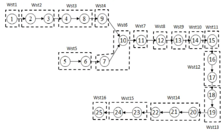
The precedence graph of the Polo-Shirt product in Table 2 is shown in Figure 2, along with a sample assignment of tasks into workstations. This sample assignment ensures that the constraints about machines in a workstation and precedence relations are satisfied.
Figure 1: Model of Polo-Shirt.
Table 2: Product technological indexes of Polo-Shirt
No Task Machine Type ti(s)
1 Check, mark
placket Check-table 1 32.0
2 Sew placket to front
Lockstitch
machine 1 30.0
3 Topstitch placket Lockstitch
machine 1 118.5
4 Trim top of
placket Hand-made 3 12.0
5 Sew collar with collar band
Lockstitch
6 Trim bottom edge of
collar band Hand-made 3 12.0
7 Trim bottom edge of
collar band Hand-made 3 10.0
8 Sew shoulder Overlock
ma-chine 1 23.2
9 Topstitch shoulder
1 needle -chainstitch machine
1 11.5
10 Sew collar band with 2 point top of placket
Lockstitch
machine 1 27.3
11 Sew collar Overlock
ma-chine 1 32.4
12 Topstitch collar band Lockstitch
machine 1 87.9
13 Attach sleeve set to armhole
Overlock
ma-chine 1 43.9
14 Topstitch armhole
1 needle -chainstitch machine
1 24.8
15 Side seam Overlock
ma-chine 1 61.4
16 Hem bottom opening
2 needles -chainstitch machine
1 30.8
17 Hem sleeve opening
2 needles -chainstitch machine
1 41.6
18 Sew bottom of placket Lockstitch
machine 1 15.4
19 Sew bottom opening, sleeve opening
Lockstitch
machine 1 23.0
20 Button hole on collar band
Button holing
machine 2 9.5
21 Button hole on placket Button holing
machine 2 19.0
22 Button Button
ma-chine 2 38.0
23 Bartack placket Bartack
machine 1 9.5
24 Bartack hem sleeve opening
Bartack
machine 1 19.0
25 Trim thread Hand-made 3 36.0
Figure 2: Precedence graph and a sample assignment of tasks into workstations.
3
Solution overview
3.1
Solution outline
To solve the GALBP-2 problem, we simply use binary search method to find the minimum cycle time. Because if there is a solution which consumes no more thanNˆ work-ers whenR=xthen the minimum value ofRis certainly not greater thanx, and if such a solution does not exist it means thatRmust be greater thanx(the correctness of this argument will be proven in section 3.2). To check for the existence of such a solution, we will have to solve a sub-problem which is also a GALBP: Given the set of all tasks, the valuesRand∆, find a way to assign tasks into work-stations in order to minimize the total number of workers.
The followingGALBP2procedure is the framework for our solution. Given the setT asksof tasks, the upper bound of number of workersNˆ and the deviation coefficient of cycle time∆,GALBP2will produce an estimated optimal solutionwstSetwhich is a set of workstations, along with its corresponding valuesR,N, andH. The return value of GALBP2has the form(R, N, H, wstSet). In this proce-dure, we assume thatis a very small real positive number,
αis the maximum processing time of a task inT asksand
β is the sum of processing time of three tasks which have largest processing time inT asks(ifM ≤ 3thenβis the sum of processing time of all tasks inT asks).
The procedure GALBP1 inside GALBP2 solves the sub-problem which is also a GALBP. It takes three pa-rameters: T asks, R and ∆. It generates a solution
Procedure 1Solve GALBP-2 Require: T asks: set of all tasks,
ˆ
N: upper bound of total no. of workers, ∆: deviation coefficient of the cycle time.
1: procedureGALBP2(T asks,Nˆ,∆) 2: lowR← α
3(1+∆) .min validR
3: upR← β
1−∆ .max effectiveR
4: whileupR−lowR > do 5: R←upR+2lowR
6: (N, H, wstSet)←GALBP1(T asks, R,∆)
7: ifN >Nˆthen 8: lowR←R 9: else
10: upR←R
11: (N, H, wstSet)←GALBP1(T asks, upR,∆)
12: ifN >Nˆthen .no solution 13: return(∞,∞,0%, N U LL)
14: else
15: return(upR, N, H, wstSet)
this procedure.
3.2
Binary search correctness
Recall that in section 3.1, we have stated that if there is a solution which consumes no more thanNˆ workers when
R=xthen the minimum value ofRis certainly not greater thanx, and if such a solution does not exist it means thatR
must be greater thanx. The correctness of this argument is proven in Lemma 3.1 below.
Lemma 3.1. Let T asks be any set of tasks and ∆ ∈ {5%,10%,15%}. Let R1, R2 such that 3(1+∆)α ≤
R1 < R2, where α is the maximum processing
time of a task in T asks. Assume that procedure
GALBP1 can always produce an accurate result, if we
set(N1, H1, wstSet1) =GALBP1(T asks, R1,∆)and (N2, H2, wstSet2) = GALBP1(T asks, R2,∆), then
N1≥N2.
Proof. First we need to show that for allR ≥ α
3(1+∆), a valid solution for GALBP1always exists. Indeed, a so-lution where each workstation contains exactly one task would fit all the constraints mentioned in the problem state-ment.
Then, we consider an interesting observation here:
wstSet1 is also a solution whenR = R2since all men-tioned constraints are still satisfied. Moreover, ifR=R2, solution wstSet1 will consumes not as many workers as itself when R = R1, because of the way we calculate the number of workers in each workstations. Assume that when R = R2,wstSet1 consumesN workers, then we haveN2≤N ≤N1which is what we want to prove.
Actually, when R < 3(1+∆)α , there will be no solu-tion. Because there exists at least one workstationiwhich hasTi >3(R+ ∆R), contradict with problem statement.
Therefore settinglowR= 3(1+∆)α at the beginning of pro-cedure GALBP2 is indeed appropriate. Moreover when
R > 1−∆β , the minimum number of workers stops to de-crease further, so initializingupR= 1−∆β is suitable too.
4
Methods to estimate the procedure
GALBP1
With the application ofGALBP2procedure, our original GALBP-2 is turned into solving another GALBP-1 in pro-cedureGALBP1. GALBP-1 is very similar to the origi-nal problem GALBP-2, with all the constraints remain the same except that the number of workers is not bound any-more.
Since the GALBP-1 in procedureGALBP1 is an NP-hard problem, it cannot be fully solved in polynomial time. Therefore, we tried to apply exhaustive search (brute-force search) along with different meta-heuristic methods such as simulated annealing (SA for short) and SA with greedy to produce answers as close as possible to the optimal ones. For a similar version of this GALBP-1 whereH must not be less than80%, we have already proposed an efficient SA algorithm [8] which performs excellently in terms of accu-racy and speed. Therefore, with some reasonable modifi-cations, we could expect our same methods to work well in this GALBP-1.
Throughout section 4, we introduce about our ap-proaches in detail to cope with this GALBP-1. The follow-ing section 5 will contain a full evaluation of all methods when being applied to solve our original GALBP-2 based on experimental results on real data of the garment indus-try.
4.1
Exhaustive search
The exhaustive search finds the optimal result by consider-ing all possible solutions. We design a simple exhaustive search algorithm for this GALBP-1 in the procedure 2.
In this procedure, wstis the current built workstation which consists of tasks, curSol is the current solution which is a set of workstations and bestSolis the current best solution. By initializing bestSol as a random valid solution and callingexhaustive(1,1,∅,∅), we will have
bestSolas our optimal solution whenexhaustive termi-nates.
Procedure 2Exhaustive search for GALBP-1 Require: i:1sttask in current workstation,
j: last added task in current workstation,
wst: current workstation,
curSol: current solution.
1: procedureexhaustive(i,j,wst,curSol) 2: ifi > Mthen
3: ifcurSolis better thanbestSolthen 4: bestSol←curSol
5: else ifwst=∅then 6: iftaskiis markedthen
7: exhaustive(i+ 1, i+ 1,∅, curSol) 8: else
9: Pushtaskiintowst
10: exhaustive(i, i, wst, curSol) 11: Poptaskiout ofwst
12: else
13: ifwstis validthen 14: Mark all tasks inwst
15: PushwstintocurSol
16: exhaustive(i+ 1, i+ 1,∅, curSol) 17: Popwstout ofcurSol
18: Unmark all tasks inwst
19: if|wst|<3then
20: fork←j+ 1toM do 21: iftaskkis not markedthen
22: Pushtaskkintowst
23: exhaustive(i, k, wst, curSol) 24: Poptaskkout ofwst
4.2
Simulated annealing
SA algorithm has been widely applied due to its feasibil-ity in NP-hard problem classes through a randomized con-trolled process with reasonable calculation time. There-fore, the SA algorithm is a good tool for ALBP with a lot of constraints.
4.2.1 Motivation and idea
Simulated annealing (SA for short) was first applied to op-timization problems by S. Kirkpatrick et al. [18] and V. Cerny [5]. In the book "Metaheuristics: From design to implementation" of El-Ghazali Talbi [28], the author de-scribed almost every aspect of SA in detail. It is a meta-heuristic to approximate optimal solution in a large search space for an optimization problem. The idea of SA algo-rithm is derived from physical metallurgy. The metal is heated to high temperatures and cooled slowly so that it crystallizes in a low energy configuration.
SA is chosen to solve this ABLP because of its simplicity and efficiency. It allows for a more extensive search for the global optimal solution, and can even find a global optimal solution if it runs for enough amount of time.
We represent our SA approach in Procedure 3. This
Pro-cedure is a close edition of the general SA algorithm from Talbi’s book [28].
Procedure 3Simulated Annealing Require: s0: initial solution,
Tmax: starting temperature,
L: neighbor generation loop time limit,
Tdec: temperature drops after each step,
P: probability to accept worse solution.
1: procedureSA(s0,Tmax, L, Tdec, P)
2: s←s0 3: T ←Tmax
4: whileT >0do 5: fori←1toLdo
6: Generate a random neighbors0
7: ifs0is better thansthen
8: s←s0
9: else
10: Assigns←s0, probabilityP(T) 11: T←T−Tdec
12: returnBest solution found
There are five parameters that we need to decide for SA:
s0as the initial solution; starting temperatureTmax, Land
Tdec for cooling schedule; andP as the acceptance
prob-ability of moving to a worse solution. Also we need to design a procedure to generate a random neighbors0from a current solutions. All these factors will affect the quality of our algorithm.
4.2.2 Initial solution
In theory, the initial solutions0 can be any valid solution and it does not affect the quality of SA. However, when the solution searching space is too large, a good initial solution can be a suitable approximation for the global optimum in a short amount of time. In section 4.2 we set a random solution as the initial solution for SA, and in section 4.3 we will assign a solution obtained from a greedy method tos0. Result comparison between these two approaches shows a remarkable efficiency difference.
4.2.3 Neighbor generation
A neighbor of a solutionsis generated simply by moving a task from a workstation to another workstation (includ-ing creat(includ-ing a new workstation consist of only that task) or swapping two tasks in two different workstations. There are at mostM2valid neighbors of a solution.
Among all valid neighbors ofs, we just consider its χ
best neighbors and randomly choose one of them. The rea-son why we do not choose among all valid neighbors is to save computation cost without worsening the algorithm efficiency too much.
range of neighbor is considered and at the end only better solutions are chosen.
4.2.4 Move acceptance
Usually, the probabilityPthat a worse solution is accepted depends on the current temperatureT, the current solution
sand the new solutions0. One of the most basic forms of
P [28] can be written as:
P(T, s, s0) =e−f(s
0)−f(s)
T =e−∆TE
In which∆E =f(s0)−f(s)is the different of quality between the new and current solution. However in our SA algorithm,Pdepends only onTby a simple formula:
P(T) =TT
max
∆E is not used in our case since the quality of sand its chosen neighbors0 are not too different, they are even very close. Becauses0is generated fromsby just moving a task from a workstation to another or swapping two tasks in two workstations, and alsos0 is chosen amongχ best neighbors ofs. Therefore,∆Etends to be very small and negligible. Also, it is very hard to find an ideal formula for calculating the quality of a solution. Any tuned formula for a solution’s quality is just overfit to some set of tests and performs badly in other tests.
Computational results show thatP(T)works well com-pared to any tuned version of P(T, s, s0)that we design. Moreover, in our caseP(T)formula is much simpler and more reasonable.
4.2.5 Cooling schedule
In theory, the higherTmaxandLare the higher chance for
optimal solution to be discoverable. Similarly, the lower
Tdec is, the better our final solution will be. However, to
save computation energy, these three parameters should be carefully tuned.
4.2.6 Multiple execution
Since the solution search space for this GALBP-1 is very large, it is not guaranteed that when SA is applied on a unique input, a unique output will be produced. There-fore, given an input, SA algorithm will be repeated multi-ple times to provide multimulti-ple answers, then the best answer among them will be the solution forGALBP1procedure. By experimenting on actual data, we realize that 10 times of repetition is enough to stabilize our SA algorithm with-out taking too much of time.
4.3
Simulated annealing with greedy
A good initial solution provided by a greedy approach can always be a suitable approximation for the optimal result in a short amount of time. Also, when the solution search space is too large, it could help SA to find better final solu-tion by focusing the process on a critical region only. With our GALBP-1, our initial solutions0for SA is constructed by a 5-step algorithm described below:
* Step 1: Choose a task usuch that there is not any remaining taskv 6= uwherevmust be done beforeuis processed.
* Step 2: Create a workstationXwhich containsuand some of the remaining tasks so that X is valid and the following W sX value is maximize (W s here stands for
"worker saved"):
W sX =n0X−nX
Wheren0Xis the total number of workers needed to com-plete all the tasks in workstationXif we divide these tasks into separated one-task-only workstations. If there are many workstations X with the same valueW sX, choose
any workstation which is balanced. * Step 3: AddXtos0.
* Step 4: Remove all tasks belong toX.
* Step 5: If there is some task remaining, go back to Step 1.
At step 2 of this algorithm, a greedy strategy is utilized: the best workstation which contains taskuis added to the solution. Such a strategy efficiently exploits a signature property of an assembly line: Its precedence graph is al-most identical to a tree with only a few number of branches. Therefore, a workstation tends to consist of connected tasks on the precedence graph, and removing them does not af-fect our future decisions so much. Indeed, experimental results which will be discussed in section 5 show that the SA with greedy solution’s efficiency is usually better than that of exhaustive search and traditional SA, in terms of both accuracy and running time.
5
Computational results
If the exhaustive search procedure were allowed to run fully, it would take several hours or even days until termi-nation which is infeasible in industrial environment. There-fore, for each test, we forced it to terminate when it is called more than6×106times recursively, and its best produced result is collected. Besides that, for all versions of SA, we setTmax = 100, L = 20andTdec = 5to guarantee
so-lution quality without consuming too much time. All al-gorithms are implemented in C++, and run on a computer which has 2.60GHz i7-8850H CPU (12 CPUs), NVIDIA Quadro P1000, 16GB RAM and 512GB SSD.
Our algorithms were tested on real data set related to the production of Polo-Shirt products at Dong Van Garment Factory, Hanoi Textile & Garment Joint Stock Corporation, Vietnam. There are 12 cases, where 6 tests are created from each of these cases by modifying∆andNˆ. The values of ∆andNˆ for each test are the combinations of three values of ∆ (5%,10%and15%) and two different values ofNˆ
whereNˆhighthe greater is about twice asNˆlowthe smaller
andNˆlow ≤1.5M. NˆhighandNˆlow are different among
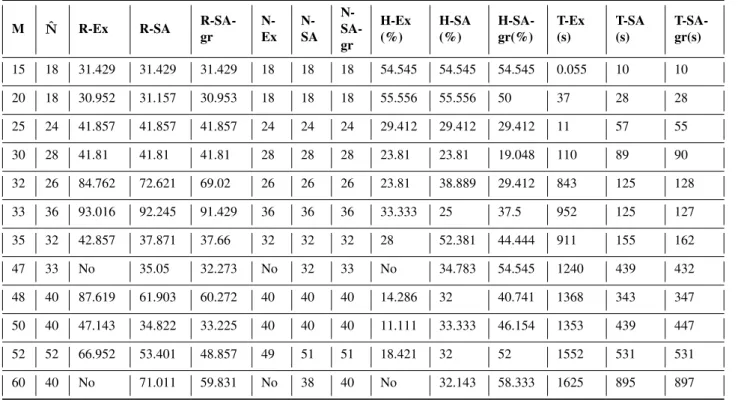
Table 3: Results for tests having∆ = 5%andNˆ = ˆNlow
M Nˆ R-Ex R-SA
R-SA-gr
N-Ex
N-SA
N- SA-gr
H-Ex (%)
H-SA (%)
H-SA-gr(%)
T-Ex (s)
T-SA (s)
T-SA-gr(s)
15 18 31.429 31.429 31.429 18 18 18 54.545 54.545 54.545 0.055 10 10
20 18 30.952 31.157 30.953 18 18 18 55.556 55.556 50 37 28 28
25 24 41.857 41.857 41.857 24 24 24 29.412 29.412 29.412 11 57 55
30 28 41.81 41.81 41.81 28 28 28 23.81 23.81 19.048 110 89 90
32 26 84.762 72.621 69.02 26 26 26 23.81 38.889 29.412 843 125 128
33 36 93.016 92.245 91.429 36 36 36 33.333 25 37.5 952 125 127
35 32 42.857 37.871 37.66 32 32 32 28 52.381 44.444 911 155 162
47 33 No 35.05 32.273 No 32 33 No 34.783 54.545 1240 439 432
48 40 87.619 61.903 60.272 40 40 40 14.286 32 40.741 1368 343 347
50 40 47.143 34.822 33.225 40 40 40 11.111 33.333 46.154 1353 439 447
52 52 66.952 53.401 48.857 49 51 51 18.421 32 52 1552 531 531
60 40 No 71.011 59.831 No 38 40 No 32.143 58.333 1625 895 897
and running time in seconds is documented to make dia-grams on Figure 3.
The top six diagrams on Figure 3 show the cycle timeR
obtained from exhaustive search, SA and SA with greedy algorithms, divide by a numberR0which is calculated as:
R0=
M
X
i=1
ti
ˆ
N (12)
R0is used as an approximation for the lower bound of
R, since if∆ = 0%thenR0 is exactly the lower bound of R and actually ∆ is quite small (∆ ≤ 15%) which means the real lower bound ofR is not so different from
R0. ThereforeR0is used to normalizeR. Among the top six diagrams, the upper three of them consist of tests hav-ingNˆ = ˆNlow and the lower three consist of tests having
ˆ
N = ˆNhigh. Each column contains a pair of diagrams
sharing a particular∆value (5%,10%or15%). The same order applies to diagrams of the balance efficiencyH and running time.
For example, Table 3 shows results of 12 tests having ∆ = 5%andNˆ = ˆNlow. Here "Ex" is exhaustive search,
"SA" is simulated annealing and "SA-gr" is simulated an-nealing with greedy. These results are used to built the top-left diagram in each set of six diagrams in Figure 3.
SinceR0is an approximation for the lower bound ofR, a value ofRis a good answer if it is not so far fromR0. WhenNˆ = ˆNlow, based on Figure 3, we can see that both
SA and SA with greedy results are as good as results of
exhaustive search in small tests but much better than ex-haustive search in medium and large tests. Even in some cases, due to early termination, exhaustive search does not provide any valid solution, as opposed to SA algorithms, which still produces quality answers for all tests. In case of Nˆ = ˆNhigh, the results ofR may not be close toR0 sinceNˆhigh ≈ 2 ˆNlow can be a bit too high which made
R0too much lower than the real lower bound ofR. Nev-ertheless, SA algorithms still show that they are always not worse than exhaustive search. In addition, SA with greedy is usually slightly better than traditional SA in terms ofR, which reveals the effectiveness of greedy initial solution.
For the balance efficiency H, SA algorithms can be slightly worse than brute force when the number of tasks
M is small. However as M grows larger, SA algorithms clearly become superior to the exhaustive one. Moreover,
H is usually higher than 40% and often fluctuates from 60% to80% when SA is utilized which are quite satisfy-ing outcomes. A point worth notsatisfy-ing is that SA with greedy is remarkably better than exhaustive search and traditional SA in almost all test cases.
In case of running time, SA algorithms completely out-perform exhaustive search as expected since they are poly-nomial time algorithms while exhaustive search theoreti-cally runs in exponential time. Also, results are produced from SA in less than 20 minutes even for the largest test cases. With its fast processing speed, SA is perfectly suit-able for real industrial environment.
Figure 3: Diagrams of cycle time (R), balance efficiency (H) and running time of exhaustive search, SA and SA with greedy on 72 tests from Dong Van Garment Factory, Hanoi Textile & Garment Joint Stock Corporation, Vietnam.
the SA with greedy version is clearly the most excellent, compared to both exhaustive search and traditional SA.
6
Conclusion
prob-lem in the garment industry. Our GALBP-2 has the primary goal of minimizing the cycle time given the upper bound of number of workers. The secondary goal is minimizing the total number of workers on the assembly line. Then the last goal is determining the maximum balance efficiency. We efficiently utilized binary search to turn the original prob-lem into a simpler probprob-lem GALBP-1, where the primary objective is minimizing the total number of workers and the secondary goal is maximizing the balance efficiency, given the cycle time. Then we introduced three methods to solve this GALBP-1: exhaustive search, SA and SA with greedy. All of them have their particular advantages in terms of accuracy and running time, depend on different test sizes. These algorithms are good supporting tools for garment factory managers to make plans before decisions. In other real assembly line balancing cases, our mentioned methods should also be considered as promising directions.
Acknowledgments
The authors would like to acknowledge the Dong Van Gar-ment Factory, Hanoi Textile & GarGar-ment Joint Stock Corpo-ration, Vietnam for supporting survey, experiment to com-plete this study.
References
[1] Ilker Baybars. A survey of exact algorithms for the simple assembly line balancing problem. Man-agement science, 32(8):909–932, 1986. https: //doi.org/10.1287/mnsc.32.8.909.
[2] Nils Boysen, Malte Fliedner, and Armin Scholl. A classification of assembly line balancing prob-lems. European journal of operational research, 183(2):674–693, 2007. https://doi.org/10. 1016/j.ejor.2006.10.010.
[3] Benjamin Bryton.Balancing of a continuous produc-tion line. PhD thesis, Northwestern University, 1954.
[4] GM Buxey. Assembly line balancing with multi-ple stations.Management science, 20(6):1010–1021, 1974. https://doi.org/10.1287/mnsc. 20.6.1010.
[5] Vladimír ˇCern`y. Thermodynamical approach to the traveling salesman problem: An efficient simulation algorithm. Journal of optimization theory and appli-cations, 45(1):41–51, 1985. https://doi.org/ 10.1007/bf00940812.
[6] James C Chen, Chun-Chieh Chen, Yi-Jhen Lin, CJ Lin, and TY Chen. Assembly line balancing prob-lem of sewing lines in garment industry. In Proceed-ings of the 2014 International Conference on Indus-trial Engineering and Operations Management Bali,
Indonesia, pages 7–9, 2014. https://doi.org/ 10.1109/icmlc.2009.5212600.
[7] Wen-Chyuan Chiang. The application of a tabu search metaheuristic to the assembly line balancing problem.
Annals of Operations Research, 77:209–227, 1998.
[8] Mai Huong Dinh, Viet Dung Nguyen, Van Long Truong, Phan Thuan Do, Thanh Thao Phan, and Duc Nghia Nguyen. Simulated annealing for the as-sembly line balancing problem in the garment indus-try. InProceedings of the Tenth International Sym-posium on Information and Communication Technol-ogy, pages 36–42, 2019.https://doi.org/10. 1145/3368926.3369698.
[9] Selin Hanife ERYÜRÜK. Clothing assembly line design using simulation and heuristic line balancing techniques. Journal of Textile & Apparel/Tekstil ve Konfeksiyon, 22(4), 2012.
[10] SH Eryuruk, F Kalaoglu, and M Baskak. Assembly line balancing in a clothing company. Fibres & Tex-tiles in Eastern Europe, 66(1):93–98, 2008.
[11] Rasul Esmaeilbeigi, Bahman Naderi, and Parisa Charkhgard. The type e simple assembly line bal-ancing problem: A mixed integer linear program-ming formulation. Computers & Operations Re-search, 64:168–177, 2015. https://doi.org/ 10.1016/j.cor.2015.05.017.
[12] Waldemar Grzechca. Assembly line balanc-ing problem with reduced number of worksta-tions. IFAC Proceedings Volumes, 47(3):6180– 6185, 2014. https://doi.org/10.3182/ 20140824-6-za-1003.02530.
[13] Allan L Gutjahr and George L Nemhauser. An al-gorithm for the line balancing problem. Manage-ment science, 11(2):308–315, 1964. https:// doi.org/10.1287/mnsc.11.2.308.
[14] WB Helgeson and Dunbar P Birnie. Assembly line balancing using the ranked positional weight tech-nique. Journal of industrial engineering, 12(6):394– 398, 1961.
[15] Thomas R Hoffmann. Assembly line balancing with a precedence matrix. Management Science, 9(4):551–562, 1963. https://doi.org/10. 1287/mnsc.9.4.551.
[16] Mahmut Kayar and Ö C Akyalçin. Applying dif-ferent heuristic assembly line balancing methods in the apparel industry and their comparison. Fibres & Textiles in Eastern Europe, 2014. https://doi. org/10.5604/12303666.1191438.
[18] Scott Kirkpatrick, C Daniel Gelatt, and Mario P Vec-chi. Optimization by simulated annealing. science, 220(4598):671–680, 1983. https://doi.org/ 10.1126/science.220.4598.671.
[19] N Kriengkorakot and N Pianthong. The assembly line balancing problem: Review problem. J. Ind. Eng, 6(3):18–25, 1955.
[20] Sophie D Lapierre, Angel Ruiz, and Patrick Sori-ano. Balancing assembly lines with tabu search. Eu-ropean journal of operational research, 168(3):826– 837, 2006. https://doi.org/10.1016/j. ejor.2004.07.031.
[21] Yuchen Li, Honggang Wang, and Zaoli Yang. Type ii assembly line balancing problem with multi-operators. Neural Computing and Applications, 31(1):347–357, 2019. https://doi.org/10. 1007/s00521-018-3834-1.
[22] Patrick R McMullen and GV Frazier. Using sim-ulated annealing to solve a multiobjective assem-bly line balancing problem with parallel worksta-tions. International Journal of Production Research, 36(10):2717–2741, 1998. https://doi.org/ 10.1080/002075498192454.
[23] SG Ponnambalam, P Aravindan, and G Mogileeswar Naidu. A multi-objective genetic algorithm for solv-ing assembly line balancsolv-ing problem. The Interna-tional Journal of Advanced Manufacturing Technol-ogy, 16(5):341–352, 2000. https://doi.org/ 10.1007/s001700050166.
[24] M. E. Salveson. Induced matchings in intersec-tion graphs. The Journal of Industrial Engineering, 6(3):18–25, 1955.
[25] Bhaba R Sarker and JG Shanthikumari. A generalized approach for serial or parallel line balancing.THE IN-TERNATIONAL JOURNAL OF PRODUCTION
RE-SEARCH, 21(1):109–133, 1983. https://doi.
org/10.1080/00207548308942341.
[26] Armin Scholl and Christian Becker. State-of-the-art exact and heuristic solution procedures for simple as-sembly line balancing. European Journal of Opera-tional Research, 168(3):666–693, 2006. https:// doi.org/10.1016/j.ejor.2004.07.022.
[27] Yuri N Sotskov, Alexandre Dolgui, Tsung-Chyan Lai, and Aksana Zatsiupa. Enumerations and stability analysis of feasible and optimal line balances for sim-ple assembly lines. Computers & Industrial Engi-neering, 90:241–258, 2015. https://doi.org/ 10.1016/j.cie.2015.08.018.
[28] El-Ghazali Talbi. Metaheuristics: from design to implementation, volume 74. John Wiley & Sons, 2009. https://doi.org/10.1002/ 9780470496916.