MODELLING AND SIMULATION OF LASER CHEMICAL PROCESSING (LCP) FOR THE MANUFACTURING OF SILICON SOLAR CELLS DISSERTATION

i

D

ISSERTATION

zur Erlangung des akademischen Grades

des Doktors der Naturwissenschaften

(Dr. rer. nat.)

an der Universität Konstanz

Fachbereich Physik

vorgelegt von

Andreas Fell

Fraunhofer Institut für Solare Energiesysteme

Freiburg im Breisgau

2010

Konstanzer Online-Publikations-System (KOPS) URN: http://nbn-resolving.de/urn:nbn:de:bsz:352-opus-122997

i

1 Introduction ...1

1.1 Motivation ...1

1.2 LCP – status of research ...3

1.3 Literature review ...7

1.4 Aims and scopes ...7

2 Mathematical modelling ...9

2.1 Overview of physical effects in LCP...9

2.2 Optics...11

2.2.1 Complex refraction index of silicon ...12

2.2.2 Absorption ...13

2.2.3 Reflection ...15

2.3 Thermodynamics ...19

2.3.1 Heat transport ...19

2.3.2 Phase change solid – liquid ...21

2.3.3 Evaporation...23

2.3.4 Species transport...25

2.4 Fluid dynamics ...27

2.4.1 Basic fluid flow ...28

2.4.2 Multiphase flow...28

2.4.3 Melting and solidification...29

2.5 Chemistry ...30

2.5.1 Photochemical radical generation...30

2.5.2 Reactions ...31

3 Fundamentals of the simulation methods ...32

3.1.1 Spatial discretization... 33

3.1.2 Time integration... 36

3.1.3 Alternating direction explicit (ADE) method ... 38

3.2 Fluent ... 39

3.2.1 Solver basics ... 40

3.2.2 User defined code – UDS and UDF... 41

3.2.3 Multiphase flow ... 42

4 Implementation... 43

4.1 Heating and radical generation in the liquid jet ... 43

4.2 LCPSim: optics and thermodynamics at the reaction spot ... 47

4.2.1 Solving of the heat transport equation ... 48

4.2.2 Implementation of the ADE method... 51

4.2.3 Treatment of the surface geometry ... 55

4.2.4 Intensity distribution, surface reflections and raytracing... 56

4.2.5 Semi analytical heat sources ... 61

4.2.6 Surface recession due to evaporation... 61

4.2.7 Diffusion of impurity atoms in silicon melt... 64

4.2.8 Multilayer implementation... 66

4.2.9 Grid generation and adaptation... 67

4.2.10 User settings and program structure... 71

4.2.11 Verification ... 73

4.3 Adaption of Fluent ... 78

4.3.1 Separate temperature fields... 78

4.3.2 Melting / solidification and density change ... 79

4.3.3 Free surface heat transfer ... 81

4.3.4 Verification ... 83

4.4 Coupling of LCPSim and Fluent... 87

5 Simulation results...92

5.1 Heating and radical generation in the liquid jet...92

5.2 Influence of basic parameters in silicon laser processing...95

5.3 Dry laser ablation...99

5.3.1 Silicon...99

5.3.2 Silicon nitride layer ...101

5.4 Ablation of silicon by LCP...102

5.4.1 Evaporation...102

5.4.2 Melt expulsion by the liquid jet...104

5.4.3 Cooling effect ...109

5.5 Dry laser doping ...111

5.6 LCP doping...112

5.6.1 Simulations with flat top profile...113

5.6.2 Influence of inhomogeneous intensity profile...115

6 Summary...122

7 Deutschsprachige Zusammenfassung...127

A Program code and settings ...132

A.1 LCPSim: start.m ...132

A.2 LCPSim: gridadapt_2d.m ...135

A.3 LCPSim: ade_2d.m...139

A.4 LCPSim: sims.m...142

A.5 Fluent: Fluent C-code for UDFs...143

A.6 Fluent: solver settings...147

B List of symbols and abbreviations ...149

C Publications...156

References ...158

1

1.1 Motivation

A major part of the current threats to the human civilisation originates from the world energy system, which is based mainly on fossil fuels. On the one hand, the limited amount of fossil and nuclear resources will lead to a dramatic increase of energy cost in the mid term, the effects of which are already clearly visible, which will have an unforeseeably great impact on world poverty and social stability. On the other hand, the air pollution by burning fossil fuels affects seriously the world’s flora and fauna, mainly due to climate change by the greenhouse effect. The greenhouse gases emitted up to now are already high enough to possibly heat up the world’s average temperature by over 2 degrees, which is treated as a critical value for non-healable climate change [1] with strongly increased weather extremes, dessert spreading, sea-level rise and so on.

Therefore one of the biggest tasks for mankind is to strongly reduce and finally completely eliminate the amount of fossils and nuclear power as primary energy in a very fast way. Besides energy savings the highest effort has to be made to develop cost efficient renewable energy usage, because only then is a rapid worldwide market introduction possible. The example of Germany showed that with a suitable political frameset, namely the EEG [2], extremely high growth rates of installed renewable power capacities can be achieved. This strong market growth at the same time increases research and development efforts, which leads to a decreasing cost of the installations. For wind power, grid parity has already been reached, even in moderately windy regions. This is now the reason for its worldwide rapid market growth even without high political support and there will be a significant contribution to world energy production in the near future.

Another promising renewable energy source is photovoltaics. The potential of usable solar radiation on earth is much greater than world energy consumption. Also, photovoltaics have shown rapid growth rates of 50% since 2003 [3], as shown in Fig. 1-1. Currently, grid parity has only been reached in very sunny regions. Therefore political support is still needed to ensure further cost reductions. In addition to cost reductions by large scale manufacturing, an important key is to introduce new technologies to increase the light conversion efficiency of a solar cell, which directly improves the cost per WattPeak ratio of the final power plant.

Fig. 1-1: World PV module production from 1990 to 2007 taken from [3]

This work was done in the field of crystalline silicon solar cells, which have the biggest market share, because of technology transfer from semiconductor industry and the higher efficiency compared to thin film technologies. It is quite well known, how to manufacture a highly efficient crystalline silicon solar cell, for example the PERC cell [4] or the back-contact cell [5]. But a great deal of necessary manufacturing steps, mainly consisting of photolithography, are too cost intensive for an industrial application. Thus world research activities in this field currently focus on the development of new cheap processes to introduce high efficiency cell structures in industry.

Within this scope lasers offer a variety of new promising applications. They work maskless, contact-free and are able to process arbitrary geometries with very high speed. A special laser application, called laser chemical processing (LCP), is currently being developed at Fraunhofer ISE. Here a laser and a liquid jet containing suitable chemicals are combined to trigger different thermochemical processes at the reaction spot. With this technique, it is for example possible to create local phosphorous doping underneath the front metal contact fingers in just one process step, which can significantly increase the efficiency of the solar cell.

This work contributes to the development of LCP by gaining an understanding of the process physics. The use of simulations enables a better interpretation of experimental results leading to more efficient selection of parameters and optimization.

Fig. 1-2: Sketch of the LCP principle

LCP is based on the LaserMicroJet™ (LMJ) technology by Synova S.A. and was developed by Richerzhagen in 1994 [6, 7]. A hair thin jet is generated by pumping water through a tiny sharp edged nozzle. Applying the correct pressures on the order of 100 bar, a constricted jet is formed, which is stable up to 1000 times the nozzle diameter and can in this way act as an optical waveguide. LMJ is mainly used for the cutting of different materials with pulsed or continuous wave (CW) high power lasers. The laser heats, melts and evaporates the work piece and the high velocity liquid jet carries away the ablated material.

LCP was introduced by Willeke and Kray [8, 9] by replacing water with solvents containing suitable chemicals, which enables a variety of combined thermal, hydrodynamic and chemical processes at the reaction spot. Since 2003 the Fraunhofer Institute for Solar Energy Systems (ISE) is the only institution developing different LCP applications for the manufacturing of crystalline silicon solar cells. Possible applications range from microstructuring, for example the opening of passivation layers or edge isolation, to wafering, which aims to cut wafers from an ingot, to local doping and metallization, which enables selective emitter and local back surface field (LBSF) formation. Two examples, the wafering and the local doping, will be discussed in the following.

Wafering

Wafering is the process of cutting wafers out of a crystalline silicon ingot. This is usually done by a multi wire slurry saw (MWSS), where thousands of parallel wires abrasively cut an

laser beam

focusing lens

nozzle hole window

pressure chamber

liquid jet

reaction spot

ingot. The MWSS is able to produce wafers with a thickness down to 150 µm, having a kerf loss of at least the same amount. The surface of the wafers is highly damaged and contaminated especially by metals from the wire. Therefore wet chemical etching and cleaning steps are needed afterwards which further increases the overall loss of silicon. This loss is very critical considering the high price of crystalline silicon.

Because in LCP the laser is focused over the whole stable jet length in the centimetre range, very deep grooves with high aspect ratios can be processed. This makes it suitable for a wafering application. Advantages in regard to the MWSS are the potential of smaller kerfs and a better surface quality, which in overall reduces the loss of silicon significantly and makes additional etching and cleaning unnecessary. LCP wafering also has the potential of silicon recycling by using suitable reactants, namely chlorine, which would further reduce the loss of silicon.

The research in this field is focused on searching for suitable laser parameters and chemical additives to achieve deep cuts with good surface quality. Progress has been published by Hopman, Mayer and Fell [10, 11]. The ability of 7 cm cutting depth has been proven and the ablation efficiency and ablation mechanism of different laser systems has been discussed in detail. Chlorine is shown to have a very high etch rate on molten and evaporated silicon but shows no etching on solid silicon, which makes it suitable to support the thermal ablation. More recently, Mayer [12] proved a positive influence on cut quality and groove shape by adding chlorine to Fluorinert FC-770 as a solvent, see Fig. 1-3. Wafering with LCP is still in the stage of fundamental research, therefore increasing understanding of the process is necessary for further development. For this the simulation results of the present work contribute to the understanding of different ablation mechanisms like evaporation and melt expulsion.

Fig. 1-3: Influence of chlorine in the liquid jet on the groove shape after LCP line scans; left: low chlorine concentration; right: High chlorine concentration [12]

Doping with LCP is already close to an industrial application. Most relevant is the selective emitter formation on p-type solar cells. For high efficiency, a lowly doped emitter with a high “blue response” is needed. But a high surface doping is needed to ensure a good contact resistance to the metal contacts. The selective emitter combines these two issues by having a lowly doped emitter and local high doping underneath the front metal contact fingers. The high doping also reduces recombination losses in the contact area, which means neutralization of electrons and holes. Therefore the high doping increases the overall efficiency significantly and cheap processes for the manufacturing of selective emitters are of great industrial interest.

Fig. 1-4: High efficiency p-type silicon solar cell structure (PERC) with selective emitter and local back surface field (LBSF)

Usually selective emitters are produced by photolithography with a lot of masking and etching steps, which is much too cost intensive for an industrial application. With LCP, a technique is proposed that can achieve local high doping in a fast single step. For n-doping, phosphoric acid is used as a liquid medium which acts as a phosphorus dopant source. The laser power melts the silicon at the reaction spot, the phosphorus is thermally atomized and it then diffuses into the silicon melt. Because the phosphorus diffusion coefficient in the silicon melt is several orders of magnitude higher than in solid silicon, precise local doping in very short melt times is possible. Pulsed lasers with pulse durations down to a few nanoseconds are sufficient to create appropriate doping. Advantages to dry laser doping processes are the nearly infinite doping source which does not have to be placed in an extra step and enables grooving and doping at the same time. A disadvantage is that melt flow by the liquid jet can

p doped base

front metal contact

passivation and antireflection layer n-doped emitter

rear metal contact passivation layer

local high p doping local high n doping

create a bad crystal quality, whereas in dry laser doping with low power, the melt resolidificates without much movement.

Solar cell results with LCP doping have been published in [13] and [14], where it is shown that with low power nanosecond laser pulses a proper selective emitter is produced. For increasing laser power, solar cell efficiency drops rapidly above a fluence threshold of

2

25 .

1 J cm as shown in Fig. 1-5. Also, for longer pulse durations no acceptable solar efficiencies can be reached. Here simulations can help to explain these phenomena by having a close look at the physical effects taking place during LCP doping.

0 0.5 1 1.5 2 2.5 3

0 2 4 6 8 10 12 14 16 18 20

fluence [J/cm²]

solar cell efficiency [%]

60 µm nozzle, 35 kHz 60 µm nozzle, 80 kHz 80 µm nozzle, 35 kHz

Fig. 1-5: Solar cell efficiencies with selective emitter produced with LCP for different parameters [14]

In addition to the selective emitter, local doping can also be applied to create a local back surface field (LBSF). As on the front side, high doping underneath the metal contacts decreases contact resistance and recombination losses. If the back side of the solar cell is contacted only locally, an appropriate passivation and reflection layer can be introduced, which reduces back side recombination losses and increases effective absorption for long wavelengths. For a standard p-type solar cell, p-type doping is needed for creating a LBSF. Boron doping is known to show the best performance, but because of low diffusion coefficients, the commonly used furnace diffusion takes very long and is therefore not industrially feasible. With LCP using a boron-containing liquid, fast local p-doping with a passivation layer opening can be achieved in a single step. First results have proven the ability of LCP to create local boron doping [15].

For modelling and simulation of material processing using a liquid jet guided laser the only work found in literature was published by Li et al. [16]. They presented a model for laser heating, melting, surface cooling and ablation of silicon by the water jet. Rather than solving fluid flow equations for melt expulsion, they assume that the melt is completely and instantaneously removed.

The basic thermal effects of LCP also occur in dry laser processing. Therefore an overview of published research in this field is given. Because in LCP laser pulse durations have to be greater than roughly one nanosecond, the reason for this is discussed later in this work, modelling of shorter laser pulses is excluded in this overview.

The simulation of laser material interaction started in the early eighties for semiconductor applications. Wood, Grigoropoulus et al. presented models for laser heating and melting of silicon combined with dopant diffusion, see [17-21]. The one dimensional models were solved by finite difference methods. Later additional effects like evaporation, gas dynamics and plasma yielding were incorporated mainly for the application of aluminium sputtering. Here several publications with finite differences methods exist for one dimensional models [22-25], and for two dimensional models with axial symmetry [26]. Ren et al. [27] presented similar modelling applied to silicon micromachining.

One step further was taken in the modelling of laser welding. For this application mostly long pulse or continuous wave lasers are used, which cause high melt flow. Thus, free surface flow of the melt is incorporated here in contrast to the publications listed above. A good overview of this field is given by Mackwood and Craver [28]. For example, Mazumder et al. developed a fully three dimensional simulation model for all relevant effects in laser keyhole welding [29]. Mazumder et al. also presented a good review of modelling of laser processing up to 1996 [30].

For the simulation of melt flow caused by a liquid jet no literature was found and is assumed to be done for the first time in the present work.

1.4 Aims and scopes

Up to the beginning of this work, development of LCP was mainly done by trial and error. LCP owns a big amount of parameters, because of the laser – liquid jet coupling. Laser parameters like wavelength, pulse duration, power and repetition rate are combined with the jet parameters pump pressure, nozzle diameter and fluid properties, and other process parameters such as working distance and pulse overlap. The quantity already shows that trial and error is not an appropriate way to search for suitable parameters. Therefore a fundamental understanding of LCP physics is necessary for efficient parameter location and optimization.

Looking carefully at experimental results to gain an understanding of the process quickly leads to the insight that the quantity and complexity of the physical effects is much too great to get conclusive and correct interpretations. Also, analytical estimations are only applicable with strong simplifications, and neglect the high degree of coupling of the different physical effects, like the interaction between thermal melting and fluid flow.

This insight was the motivation to start numerical simulation of LCP. Multiphysics simulations give the unique possibility to observe arbitrary quantities during the process at arbitrary points in time. The present work aims to describe the coupled physical effects not in an exact quantitative, but more qualitative and efficient way. This means basically looking at the interaction of different physical effects, identifying dominating effects and observing the influence of process parameters. Although some effects can be described precisely, especially because silicon is a well known material, at very high temperatures the applied models are not fully valid and the material properties can only be estimated. Therefore using simulations for accurate quantitative forecasts is too challenging at least for moderate to high laser power. The first step for building simulation code is to choose proper mathematical models for the physical effects. Solving the resulting equations is not trivial, because of the high degree of interaction and the extreme scales of the corresponding physical quantities. For example laser light absorption can occur on a scale of a few nanometres, resulting in very high temperature gradients at the free surface of the melt. Currently no commercial simulation software is known to solve all of the relevant effects simultaneously. Therefore self programmed code is necessary to implement adopted solvers and enable transient coupling of the equations. However, the commercial software Fluent is used for simulation of fluid flow. Basic programming of a suitable fluid flow solver would have been too extensive for the timeframe of this work, whereas the use of Fluent enables a fast and efficient problem setup.

LCP can be seen as an extension of dry laser processing, because the basic effects of dry laser processing take place in LCP in rather the same way. This means that simulation of LCP can benefit from previous work done in the field of dry laser simulation, as discussed above, and that the simulation code generated in this work can widely be applied to dry laser processing. The thesis consists of four main chapters following this introduction. In the next one the theory of the physical effects taking place in LCP is described and the corresponding mathematical models are shown. The third chapter deals with the fundamentals of the numerical methods used in this work. A detailed description of the implementation of the mathematical models to program code is given in chapter four. Finally simulation results are shown for comparison with experiments and for interpretation of LCP results with respect to solar cell manufacturing.

9 This chapter deals with the mathematical description of the physical effects in LCP. The effects are summarized in optics, thermodynamics, fluid dynamics and chemistry. Suitable models are taken from literature and are applied to the silicon case. The material properties of silicon used in the simulations are also given within the description of the corresponding models.

2.1 Overview of physical effects in LCP

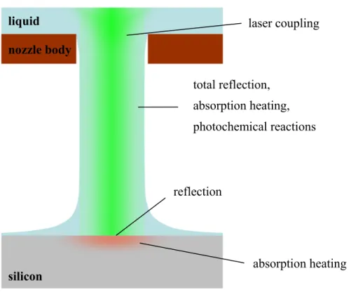
Fig. 2-1: Effects at the beginning of the laser pulse before the onset of melting and evaporation

laser coupling

total reflection, absorption heating, photochemical reactions

reflection

absorption heating

silicon liquid nozzle body

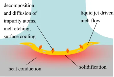
Fig. 2-2: Effects during the laser pulse after the onset of evaporation

Fig. 2-3: Effects after the laser pulse and after reattaching of the liquid to the silicon

In Fig. 2-1 to Fig. 2-3 the important effects occurring in LCP during one typical laser pulse are illustrated. First of all the liquid jet is generated by a sharp edged nozzle and shows a typical diameter of 0.83 times the nozzle opening diameter [11], confirmed by Fluent simulations performed for the present work. A laser beam is focused on the nozzle opening plane and is guided within the liquid jet via total reflections. The laser light already interacts with the jet, either by absorption heating or by photochemical reactions. This could be potentially used for generating radicals, which are generally much more reactive. The jet acts as an optical multimode waveguide. Therefore the intensity distribution in the cross section is not flat, but shows several interference peaks depending on nozzle diameter and coupling optics [31]. Reaching the surface, the laser light is partly reflected and the remaining intensity is absorbed by the silicon and acts this way as a volumetric heat source. Once the melting temperature is reached, a phase change to liquid takes place. Upon further heating, the silicon starts to evaporate. For fast evaporation, a dense vapour plume is produced, which exerts a

heated zone melt

vapour / plasma plume

evaporation, recoil pressure Etching of vapour, plasma shielding, thermal decomposition

liquid jet driven melt flow

heat conduction solidification decomposition

and diffusion of impurity atoms, melt etching, surface cooling

higher power, the dense vapour is ionized into a plasma phase, which shields significantly the laser power. After the laser pulse, the vapour partly condenses and is carried away by the liquid jet. Because the melt time is much longer than the pulse durations typically used in LCP, the liquid jet attaches again to the melt after the laser pulse and starts expelling it by the liquid jet pressure and viscous drag. At the interface to the silicon melt also evaporation of the liquid takes place resulting in a small vapour film. This film reduces the viscous forces between the silicon melt and the liquid and acts as a thermal insulation layer. Chemical reactions can take place in the liquid jet as well as at the reaction spot. In the case of silicon etching by chlorine the highest etch rates are assumed for silicon vapour, and still significant etching on silicon melt, whereas the etching of heated solid silicon is negligible [10].

The present work deals mainly with low to mid laser intensities not much above the melting threshold, so plasma effects do not have to be considered. In addition, the expansion of the vapour plume and the resulting recoil pressure and condensation effects are not yet considered. This is reasonable at least for fairly long pulse durations, because the liquid jet pressure is exerted much longer on the melt than the recoil pressure and therefore dominates the movement of the melt. For shorter pulse durations in the low nanosecond scale, the laser intensity and therefore the evaporation velocity and the recoil pressure is very high, whereas the melt time is too short for significant expulsion by the liquid jet. This means that for higher power nanosecond laser pulses the vapour phase has to be considered for a correct modelling of the ablation mechanism.

2.2 Optics

The optical effects can be categorized into absorption and reflection effects. They are modelled by geometrical optics, because the laser light can be well approximated by directional beams. The basic optical material property is the complex refraction index _n*_,

where the imaginary part k is called the extinction coefficient. k

i n

n* = − ( 2-1 )

Measurements of the refraction index for solid silicon can be found in literature. For liquid silicon only very few data exists and therefore a theoretical model, the Drude model, is used to calculate the optical properties. The wavelengths investigated in this work are 1064 nm, 532 nm and 355 nm, because these correspond to the Nd:YAG laser wavelengths used in experiments.

2.2.1 Complex refraction index of silicon

For solid silicon, measured data for the optical properties has been taken from literature [32-34] and have been fitted to the expressions shown in Tab. 2-1.

λ [nm] n [33] k [32, 34]

1064 3.56₊3.142_e−4_T[_K] _1.27e−14_T[K]4

532 3.95₊5.68_e−4_T[_K] _⎟

⎠ ⎞ ⎜

⎝ ⎛

−

K T e

430 exp 1252

.

2 2

355 5.856₋8.263_e−4_T[_K] _2.9

Tab. 2-1: Solid silicon refraction index calculated from literature data

For liquid silicon no suitable measurements for the optical properties were found, therefore the Drude model is used as described in [35]. Liquid silicon can electronically be treated as a metal, because the same characteristic free electron gas exists. The optical properties are strongly dependent on the electrical ones, because incoming photons are mainly absorbed by the free carriers. Drude gave an expression for the frequency dependent complex permittivity of a free electron gas.

( )

₍

₎

* ₁

γ ω ω

ω γ γ

ω ω ε

+ +

+ −

= pl pl

i

f ( 2-2 )

The plasma frequency ω_pl is a material specific constant value and the collision rate γ is a temperature dependent value as proposed in [36].

λ π

ω = 2 c

m m

T T γ

γ =

( 2-3 )

This results in a permittivity dependent on temperature and frequency. The required optical properties are related to the permittivity by the complex equation ( 2-4 ).

to _=2.50e16 _s−1 p

ω and _=4.7170e15_s−1 m

λ .

2.2.2 Absorption

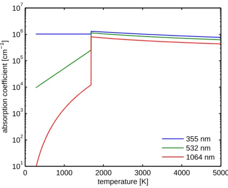
Laser light absorption occurs due to excitation of atoms or molecules by the photon energy. For the laser wavelengths used, photons interact most dominantly with electrons. This means that one photon gives all its energy to one electron. For non-free electrons not all energy levels are allowed, therefore the absorption coefficient is strongly dependent on the electronic structure of the material and the wavelength. For example for the semiconductor silicon wavelengths near or above the band gap are weakly absorbed. Increasing temperature increase also the amount of free electrons, therefore the absorption coefficient is strongly increased, which can be seen in [32].

For high laser intensities, i.e. for high photon densities, the probability that more than one photon hits an electron is increased. This is called multiphoton absorption. The absorption coefficient is then dependent on the laser intensity. Further increase of the intensity leads to more free electrons, which absorb more laser light, leading to a further ionization. At a certain intensity level this ends up in avalanche ionization, called optical breakdown, where suddenly all of the light is absorbed. It is obvious that for LCP the optical breakdown has to be avoided in the liquid jet. Therefore only laser intensities can be used in LCP, which are below the optical breakdown threshold. For the wavelengths 1064 nm and 532 nm, this threshold in water is at roughly _{100GW cm}2 _{[38]. For a 50µm jet diameter and a typical pulse energy of}

mJ

1 this would mean a critical pulse duration of roughly one nanosecond. Generally spoken for LCP applications the laser pulse durations have to be at least in the nanosecond scale. Because of this restriction, multiphoton absorption in the silicon can also be neglected. It shows neglibible absorption coefficents for the allowed intensities, which can be derived from [39].

The basic quantity for modelling absorption effects is the absorption coefficient α , which can be calculated out of extinction coefficient and the wavelength of the light.

λ π

α = 4 k ( 2-5 )

Laser light can be seen as unidirectional light. Even after crossing the surface and diffusing the light this approximation is feasible, because the absorption length is much smaller than the typical lateral width of the spatial intensity distribution. Therefore the absorption equation can be expressed in one dimension.

I dz

dI _{=−α ( 2-6 )}

If the absorption coefficient is constant over the z-coordinate, equation ( 2-6 ) can be solved analytically. The solution shown in equation ( 2-7 ) is called the Lambert-Beer law.

( )

(

)

I = _z=0exp −α ( 2-7 )

In Fig. 2-4 the temperature dependent absorption coefficient of solid and liquid silicon at various wavelengths is shown.

0 1000 2000 3000 4000 5000

101 102 103 104 105 106 107

temperature [K]

absorption coefficient [cm

−1

]

355 nm 532 nm 1064 nm

Fig. 2-5: Path enlargement by total reflection in the liquid jet

In the liquid jet another effect has to be considered. Because the laser light is coupled under an angle determined by the coupling optics, it partly travels not directly through the liquid jet as illustrated in Fig. 2-5. This results in an optical path enlargement depending on the angle between the actual light beam and the z- coordinate ϕ_beam. The relative path enlargement δ is calculated by equation ( 2-8 ).

beam

ϕ δ

cos 1

= ( 2-8 )

The maximum angle allowed is determined by the critical angle to ensure total reflection. For water as surrounding medium the maximum relative path enlargement is δ_water,max =1.335. In the simulations the path enlargement is implemented by an effective absorption coefficient.

α δ

α_eff = ( 2-9 )

2.2.3 Reflection

Reflection on the surface plays an important role in modelling of LCP, because it determines how much energy is coupled into the material. The amount of the non reflected laser light intensity is defined by the reflectivity R.

beam

ϕ

lens

nozzle opening

(

)

surf R I

I = 1− ( 2-10 )

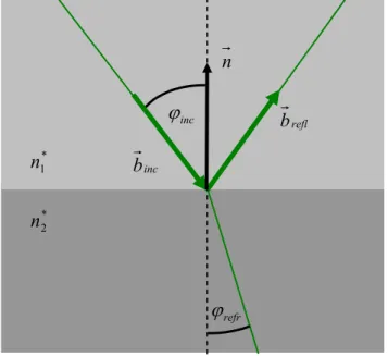
A general beam reflection at an interface between material 1 and 2 is illustrated in Fig. 2-6. For a general angular reflection, the light beam has to be distinguished in a vertically and horizontally polarized part. The regarding reflectivity is then calculated by the Fresnel formulas ( 2-11 ) and ( 2-12 ) [40].

Fig. 2-6: Beam reflection at a flat interface between material 1 and material 2

( )

( )

( )

( )

⊥ ( 2-11 )

( )

( )

( )

( )

= ( 2-12 )

The angle of refraction ϕ_refr is defined by the refraction indices and the incident angle ϕ_inc.

⎟⎟ ⎠ ⎞ ⎜⎜ ⎝ ⎛ = − inc refr n n _ϕ

ϕ sin _* sin

2 * 1

1 _{( 2-13 )}

For an arbitrary incident beam direction and an arbitrary surface normal direction the direction of the reflected beam can be calculated by the vector equation ( 2-14 ).

inc ϕ refr ϕ * 1 n * 2 n inc b refl b n

(

)

brefl = inc −2 ⋅ inc ( 2-14 )

In this case the incident angle is defined by the scalar product of surface normal and incident beam direction.

(

)

inc = −n⋅b

−1

cos

ϕ ( 2-15 )

In many cases the incident laser beam can be treated as perpendicular to the surface, i.e. when the ablated geometry shows no significant steepness. Furthermore, the surrounding medium is in our case transparent, which means that the extinction coefficient of the surrounding medium can be set to zero. The general Fresnel formulas then simplify to the well known reflectivity equation ( 2-16 ) independent of polarization.

(

)

(

)

2 2 2 1

2 2 2 2 1

k n n

k n n R

+ +

+ −

= ( 2-16 )

The resulting perependicular reflectivity for silicon is plotted in Fig. 2-7 for air and water as surrounding medium.

0 1000 2000 3000 4000 5000

0.2 0.3 0.4 0.5 0.6 0.7 0.8

temperature [K]

reflectivity

355 nm

532 nm 1064 nm

A special treatment is needed for reflection at small films, like passivation layers on the front side of a silicon solar cell. Here multi-reflections between the material interfaces take place, which can be calculated for perpendicular incident light and a non-absorptive film material to an effective reflectivity [41].

( )

( )

δ _{( 2-17 )}

1 1 * , 1 n n n n r f f f ₋ − = f f f n n n n r − − = _* 2 * 2 * 2 ,

( 2-18 )

Here δ_f is the optical path difference depending on wavelength, film refraction index and film thickness d_f .

λ π

δ f f

f

d n 4

= ( 2-19 )

Fig. 2-8: Sketch of multiple reflections at thin films.

1 n * 2 n f n * , 1f r * 2 , f

The modelling of thermodynamic effects in LCP incorporates heat transport, phase changes and species transport due to evaporation or diffusion.

2.3.1 Heat transport

As described before in section 2.2.2 the laser power is dominantly absorbed by the electrons. Before a uniform temperature for the electrons and the lattice is reached, the excited electrons have to transfer energy to the lattice. This relaxation happens on a picosecond timescale [35], which is much shorter than the used laser pulse durations of at least a few nanoseconds. So for simulation of LCP only one equal electron-lattice temperature field needs to be considered. The general partial differential equation for transient heat transport ( 2-20 ) consists of a transient, a convection, a conduction and a source term. The convection term takes into account transport of heat due to material movement like the melt flow. The source term corresponds to the absorbed laser power, see equation ( 2-21 ).

(

)

(

)

(

)

dt

d _{ρ + ∇ ρ =∇ ∇ + ( 2-20 )}

I

S_h =α ( 2-21 )

For the description of heat transport in the liquid jet the spatial distribution of the temperature in the cross section area is approximated to be constant, so equation ( 2-20 ) can be reduced to the jet direction, i.e. the z-coordinate. This is feasible because of the high length to width ratio of the liquid jet on the order of a thousand, which leads to relatively high lateral heat conduction and temperature homogenization. Also the intensity profile is varying with jet length, which results in lateral homogenization by averaging. Furthermore, the velocity profile of the liquid jet is approximately flat [42] and so the velocity is only dependent on the

z-coordinate. The heat capacity c_p, the density ρ and the heat conductivity K are assumed to be constant, so they can be placed in front of the derivatives resulting in equation ( 2-22 ).

h z

p

p S

dz T d K dz dT v c dt dT

c +ρ = 2₂ +

ρ ( 2-22 )

The heat transport in silicon is described by the enthalpy-based heat transport equation ( 2-23 ), where the enthalpy is the inner energy density in units of energy per volume. This formulation is used as proposed, for example, by Grigoropoulus et al. [21]. During phase

changes the temperature stays constant whereas the enthalpy is steadily changing, which is beneficial for implementation of a stable numerical time integration. Furthermore, for the implementation of the heat transport equation in silicon, no movement of silicon, i.e. melt flow, is considered, so the convection term can be removed.

(

)

dt

dH _{=∇ ∇ + ( 2-23 )}

In equation ( 2-23 ) the temperature needs to be calculated from the enthalpy values. This dependency is defined by the integral ( 2-24 ) for arbitrary temperature dependent thermal properties.

( )

_∫

H

0 ρ

( 2-24 )

Due to phase changes, this integral is defined only stepwise. For solid silicon the temperature dependent heat capacity and density is taken from [43]. The data has been extrapolated to show a zero enthalpy value at the absolute zero point. This dependency is not physically correct, but does not affect the calculation of the temperature field above room temperature. Additionally, this formulation shows a better numerical convergence than setting the enthalpy to zero at room temperature. A fit was performed to achieve a second order polynomial for the temperature enthalpy relation of solid silicon with 17 6 2

1 2.375e Km J

c =− − ,

J m K e

c 7 3

2 =5.512 − and c3 =98.06K. A plot of the relation ( 2-25 ) is shown in Fig. 2-10. 3

2 2

1H c H c

c

T_s = + + ( 2-25 )

Another heat transport effect is the surface cooling, which can occur by radiation and combined conductive and convective cooling. At the hot silicon surface, the radiation heat loss is determined by the Stefan-Boltzmann law neglecting the incoming radiation ( 2-26 ).

(

)

env surf T

surf T T

J =ε σ − ( 2-26 )

For conductive cooling or combined conductive and convective cooling, the surface heat transfer is approximately linearly dependent on the temperature difference of the two neighbouring materials. This can described by the heat transfer coefficient ht.

(

)

surf ht T T

J = − ( 2-27 )

The heat transfer coefficient is dependent on the thermal material properties, and for convection cooling, also on the velocity field of the cooling fluid. This means that for a specific setup the unknown heat transfer coefficient has to be derived either from measurements or calculations. In the case of cooling by a liquid impinging jet, some data can be found in literature [44], but can not be applied to the LCP case because of different jet types and different parameter values, especially Reynolds numbers.

There is also the possibility to calculate the combined convective and conductive surface heat transfer if the near surface temperature distribution is known. For this the solid side temperature gradient has to be much smaller than the fluid side one, which is the case for the interface between solid or molten silicon and the liquid medium. Then the surface heat transfer is calculated by the fluid side temperature gradient and fluid heat conductivity.

fluid surf fluid

surf

n d dT K J

,

= ( 2-28 )

Fig. 2-9: Sketch of combined convection conduction surface heat transfer

2.3.2 Phase change solid – liquid

Melting and solidification occurs if the enthalpy reaches the melting point of the processed material. In the dynamic description of the phase change the speed of the moving liquid – solid interface is dependent on the temperature difference between the interface temperature and the melting temperature [20], shown simplified in equation ( 2-29 ).

v T

n d

dT 0

env

T fluid

( )

⎜ ⎝ ⎛

⎟⎟ ⎠ ⎞ ⎜⎜

⎝

⎛ −

− − Κ

=

sl m sl m B

m sl

sl

T T T T k

L T

v 1 exp ( 2-29 )

This means, that the phase change takes place not exactly at the melting temperature, but some superheating or undercooling is needed. The kinetic rate constant Κ for melting is generally much higher than for solidification, because of the high activation energy for crystallization. In the simulations of the present work solidification velocities show values not higher than 5m s. Using the data reported in [45] results in a maximum undercooling of

K

75 . This work aims to approximately describe the physical effects rather than giving highly exact solutions, so this amount of undercooling is feasible to neglect. The superheating for melting is even lower, so for the present work the phase change solid – liquid is assumed to take place exactly at phase change temperature. In addition, the solidification speeds are lower than the critical value for amorphization of silicon of 15m s reported in [45]. This ensures that the silicon solidifies to a crystal rather than to an amorphous state for any LCP parameters.

Assuming a defined melting point, the phase change can be described by an enthalpy based approach. Once the melting temperature T_m is reached, the temperature stays constant while the enthalpy further in- or decreases until the latent heat of melting L_m has been overcome. For silicon the latent heat of melting is taken from [46] to L_mol,m =50kJ mol. Because the variable to be solved for heat transport is the enthalpy in units of energy per volume, the latent heat has to be adopted according to equation ( 2-30 ).

M L

L= _mol ρ ( 2-30 )

In the liquid state the product of heat capacity and density of silicon shows a constant value of

3 6

432 .

2 e J m

c_p =

ρ [21]. This results in the linear relation ( 2-31 ) between enthalpy and temperature with c₄ =1 ρc_p and c₅ =T_m −(H_m +L_m) ρc_p , shown in Fig. 2-10. H_m is the enthalpy where melting starts, and is calculated by inserting T_m in equation ( 2-25 ).

5

4 H c

c

For the second phase change liquid – vapour of silicon two different models are used, mainly dependent on the speed of evaporation. For low evaporation speed, i.e. for relatively low laser intensities, the material evaporates by so called normal boiling [47]. Here the evaporation takes place exactly at the boiling temperature, so an enthalpy based description as discussed above can be used. This means that the material is assumed to be fully evaporated if the boiling point at H_v is reached and additionally the latent heat of vaporization L_v has been overcome. According to [47], this model is valid for laser pulse duration of greater than roughly one microsecond.

For higher laser light intensities, significant superheating occurs and can no longer be neglected. Therefore a dynamical description of the phase change is required, which means a calculation of the evaporation speed. For nanosecond laser pulses usually the Hertz-Knudsen equation ( 2-32 ) is used. Here the evaporation rate of atoms is set to the effusion rate derived from statistical thermodynamics [48].

lv B a sat

T k m

p n

π 2

=

& ( 2-32 )

To calculate the surface recession velocity v_lv, equation ( 2-32 ) has to be divided by the atom density of the liquid ρ_l m_a . In addition it is assumed that the material does not evaporate into vacuum, but directly above the liquid surface a small layer of pure vapour exists, which is feasible within the laser pulse duration. The evaporation speed is then approximately calculated by the difference of saturation pressure and partial pressure at the surface. In this work no vapour dynamics are modelled and the partial pressure is set to an externally calculated value p_ext. This way an environmental pressure or a pressure distribution caused by the impinging jet can be taken into account.

a lv B l

ext sat lv

m T k

p p v

π

ρ 2

− =

( 2-33 )

Equation ( 2-33 ) results generally in an increasing evaporation speed with temperature, because the saturation pressure is strongly dependent on temperature. For the case of silicon no measured data for the saturation pressure above the boiling point exists, so the Clausius-Clapeyron equation ( 2-34 ) is used assuming a constant molar latent heat of vaporization

v mol

L _, . For silicon L_mol,v is calculated by the data given in [49] to 400kJ mol at the boiling point.

⎟ ⎟ ⎠ ⎞ ⎜

⎜ ⎝ ⎛

⎟⎟ ⎠ ⎞ ⎜⎜

⎝ ⎛

− −

=

b v

mol sat

T T R L p

p ₀exp , 1 1 ( 2-34 )

For reasons of energy conservation, the latent heat of vaporization has to be considered additionally as a surface heat flux during evaporation.

v L

q_lv = _v ( 2-35 )

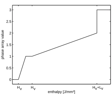
In Fig. 2-10 the entire relation of temperature and enthalpy for silicon as used in the present work is shown. Beyond the boiling point the horizontal curve corresponds to the normal boiling model, whereas for the Knudsen evaporation the further increasing curve illustrates the effect of superheating.

Fig. 2-10: Temperature – enthalpy relation as used in the simulations; the dashed curve corresponds to the superheating for the Knudsen evaporation model and the solid one to the enthalpy based model

The Knudsen evaporation as described above is still a quite simplified model, because the influence of the surrounding vapour is not considered. Especially for higher laser intensities the generated vapour plume results in high recoil pressures and directly influences the evaporation speed. A good model would be the so called Knudsen layer as proposed by Knight [50]. Here it is considered that the temperature and the pressure in a small layer above

so

lid

liquid

0 10 20 30 40 50

0 500 1000 1500 2000 2500 3000 3500 4000 4500 5000

enthalpy [J/mm³]

But using this model would require a coupled solving of gas dynamics, which is not done within the present work. Also condensation can not be calculated without gas dynamics, because the actual partial pressure at the surface has to be known.

2.3.4 Species transport

Two different effects of species transport are modelled. One is the transport of chemical additives in the liquid jet. Here mainly the light induced generation and transport of chlorine radicals is of interest. At the reaction spot the diffusion of impurity atoms in the liquid silicon is modelled, because this is the basic mechanism for the doping process.

The general transient species transport equation ( 2-36 ) includes similar to the heat transport equation a convection, a conduction and a source term. The variable to be solved is the concentration of species particles C.

sp

S C D C v dt

dC _{+ ∇ = Δ + ( 2-36 )}

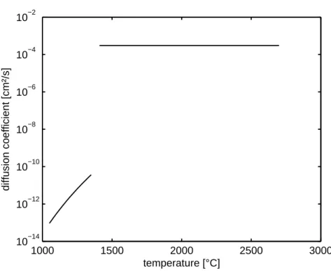
In solid silicon the diffusion coefficient is strongly temperature dependent. Usually time scales of hours are needed to diffuse a typical phosphorous emitter for silicon solar cells. For liquid silicon an increase of the diffusion coefficient of several orders of magnitude takes place, which is shown for phosphorous in Fig. 2-11 with data taken from [51] for solid silicon and [19] for liquid silicon respectively. This jump is the reason why even within the very short melt times below one microsecond produced by laser pulses, a usable amount of impurity atoms diffuses into the silicon. On the other hand, this jump clearly allows for the solid state diffusion to be neglected in the modelling of laser doping. The liquid silicon diffusion coefficient is assumed to be constant. Because liquid phase diffusion is dominated by the size of the impurity atom [48], which is temperature independent, this approximation is feasible. The melt is during its lifetime dominantly at melting temperature as shown later in this work. This further reduces the error of the final species distribution introduced by the simplified temperature independent diffusion coefficient.

1000 1500 2000 2500 3000 10−14

10−12 10−10 10−8 10−6 10−4 10−2

temperature [°C]

diffusion coefficient [cm²/s]

Fig. 2-11: Temperature dependent diffusion coefficient of phosphorous in solid and liquid silicon

If flow is not considered, the convection term in equation ( 2-36 ) can be removed. Also in the material volume no sources for impurity atoms are present. These simplifications result in the well known Fick’s law ( 2-37 ), which is used to calculate impurity atom diffusion in silicon melt.

C D dt

dC _{= Δ ( 2-37 )}

Different boundary conditions for species transport are used in this work. They can be divided into isolating, infinite source and finite source. For the isolating case no species flux over the boundary is allowed, which is for example the case at the liquid – solid interface in silicon.

0

=

surf

n d

dC _{( 2-38 )}

The infinite source boundary condition is used at the liquid jet outlet and at the silicon surface if an unlimited dopant source is assumed.

bc

surf C

section 5.5. This has to be modelled by a finite source boundary condition. Here a surface concentration dependent on the loading Θ, which transiently decreases by the dopant flux through the surface, is used. Because no suitable physical model was found, a linear relationship starting from saturation concentration in silicon melt at full loading and decreasing to zero at zero loading is assumed, see equation ( 2-40 ). Comparing the simulation with experimental results shows that this approximation describes the doping by a precursor layer source in a reasonable way.

0

=

Θ Θ =

t sat

surf C

C ( 2-40 )

For doping with LCP an infinite source boundary condition is used. The surface concentration is a free parameter and is adjusted in the simulation to fit the experimental results. Much better would be a boundary condition which can be calculated by the dopant concentration in the liquid jet. The first idea, that this surface concentration is equal or proportional to the dopant concentration in the liquid jet, gives no suitable results. Here the surface concentration of the measured doping profiles should be proportional to the dopant concentration of the solvent, which is not the case for the different measured doping profiles. Therefore, the processes at the solvent – silicon interface has to be modelled in more detail. This means considering the thermal atomization of the dopant and the dopant transport by diffusion and convection in the near interface region. This could not be done within the timeframe of the present work, so the surface concentration remains as a free parameter for LCP doping simulations.

The optical properties of silicon are generally influenced by the doping level. This is not considered in the present work, because no data has been found in literature which covers the needed concentration and temperature range. This is assumed to introduce a negligible error, because the laser light interacts mainly with the lowly doped silicon bulk, and in the liquid phase the absorption is nevertheless very high.

2.4 Fluid dynamics

For simulation of fluid flow the commercial software Fluent is used. The models and regarding equations shown in this section are taken from the Fluent manual [52], where references to literature are included.

2.4.1 Basic fluid flow

The flow to be simulated occurs on a small micrometer scale, but the Knudsen number stays well below 0.01, even for extreme assumptions for pressure and temperature. This means that the mean free path is much lower than the typical length scale, which allows for continuum flow equations to be used. These are the Navier Stokes equations consisting of conservation laws for momentum ( 2-41 ) and mass( 2-42 ), where the latter is called the continuity equation.

( ) ( )

( )

dt

d _{ρ +∇⋅ ρ =−∇ +∇⋅τ + ( 2-41 )}

( )

dt

dρ _{+∇⋅ ρ = ( 2-42 )}

The stress tensor τ accounts for viscosity effects.

⎥⎦ ⎤ ⎢⎣

⎡ _{− ∇⋅}

⎟ ⎠ ⎞ ⎜

⎝

⎛_{∇ +∇}

= v vT vE

3 2 μ

τ ( 2-43 )

Turbulence can occur in LCP because of the high velocity of the liquid jet. It is hard to choose a suitable turbulence model and parameters, especially because of the transient geometry change during expulsion of the silicon melt. In addition, this work is not aiming for exact solutions, therefore turbulence is not considered. The silicon melt is treated as an incompressible fluid, optionally with a temperature dependent density.

Because no vapour phase is simulated, the recoil pressure on the melt surface is not known and can not be considered. Especially for short laser pulses the recoil pressure can reach very high values of up to the order of 1GPa [25], which is far above the liquid jet pressure. However, the recoil pressure only takes place during the evaporation, whereas the liquid jet exerts pressure during the whole melt duration, which is significantly longer. This means that for relatively long pulse durations and low pulse energies the liquid jet induced melt flow dominates the melt flow by recoil pressure. The results of this work indicate that this is the case for melt durations greater than one microsecond.

2.4.2 Multiphase flow

Multiphase flow means considering the flow of different fluids which possess different fluid dynamic properties. Multiphase models can be basically divided into Euler-Lagrange and

for discrete particles interacting with a continuous flow field. In the Euler-Euler model, two or more interpenetrating continuous flow fields are considered. In LCP mainly the flow of the liquid jet interacting with the silicon melt is of interest, which corresponds to the Euler-Euler model. Silicon melt and liquid solvents are treated as immiscible fluids, therefore a sharp interface exists and surface tension has to be taken into account.

In the Fluent simulations the so called volume of fluid (VOF) model is used, which is a simplified Euler-Euler approach. The volume fraction a is introduced, which corresponds to the volumetric occupation of the regarding phase. At every point in space the volume fractions of all phases have to sum to one.

∑

=

= np q

q

a

1

1 ( 2-44 )

The fluid flow equations are solved for the mixture phase, where the mixture properties are defined by the volume fraction weighted average as shown in equation ( 2-45 ).

∑

=

= np

q q q

mixt a

1

ξ

ξ ( 2-45 )

(

)

(

)

dt d

, = ⋅

∇

+ ρ

ρ ( 2-46 )

Additionally the volume fraction equation ( 2-46 ) has to be solved for each phase q besides the primary phase, which allows tracking of the phase interfaces. The volume fraction of the primary phase is calculated by equation ( 2-44 ). The source term of the volume fraction equation corresponds to mass sources and to mass transfer between two phases. Because of solving only one flow field, the VOF model requires a low computational effort and is predestined for the tracking of sharp interfaces. The VOF model further allows the consideration of surface tension, which plays a significant role in LCP because of the high surface tension of silicon of 0.765N m at the melting point [53].

2.4.3 Melting and solidification

The melting and solidification model has to account for the transient change of a materials aggregate state between liquid and solid. For this the temperature dependent liquid fraction β is introduced. Fluent usually solves for temperature as the independent variable and a sudden

solidification at the exact melting temperature would cause numerical problems. Therefore a mushy region ΔT_m is defined around the melting point, where the material is linearly changing from solid to liquid.

⎟ ⎟ ⎟ ⎟ ⎠ ⎞ ⎜

⎜ ⎜ ⎜ ⎝ ⎛

⎟ ⎟ ⎟ ⎟ ⎠ ⎞ ⎜

⎜ ⎜ ⎜ ⎝ ⎛

Δ Δ − −

=max min 2 ,1 ,0

m m m

T T T T

β ( 2-47 )

To hinder movement in the solid state, a very high momentum sink is added to equation ( 2-48 ). The sink is dependent on the liquid fraction in such a way that for a liquid fraction of one, the value of the sink is zero. The nonlinear expression is optimized for numerical stability.

(

)

Smom ₃ 5

2

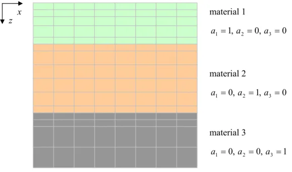
1 001 . 0 1

+ − =

β

β _{( 2-48 )}

2.5 Chemistry

Chemical effects modelled in the present work comprise photochemical decomposition of molecules and reaction kinetics. The focus is on effects in the liquid jet, mainly the generation and recombination of chlorine radicals. At the reaction spot extreme conditions in terms of time scale and temperature occur. Here no suitable data for surface reaction kinetics exists, which makes a quantitative simulation impossible.

2.5.1 Photochemical radical generation

If photon energies are high enough, the laser light is able to crack molecule bonds. This can be used to produce chlorine radicals out of molecular chlorine in the liquid jet. The amount of radicals generated equals the product of quantum efficiency Φ_d and the amount of photons absorbed by the molecular chlorine, which is the absorbed laser power divided by the photon energy [54].

c h

I S_Cl =Φ_d αCl2 λ

⋅ ( 2-49 )

The absorption coefficient of molecular chlorine is calculated by the collision cross section

c

c Cl

Cl C σ

α ₂ = ₂ ( 2-50 )

Data for chlorine radical generation with λ =355nm has been taken from [54] to Φ_d =0.35 and _1.94e 19_cm2

c

−

=

σ .

2.5.2 Reactions

Many reactions can take place during LCP, for example etching and oxidation of hot silicon, thermal decomposition of dopant sources and reactions of chemical active additives in the liquid jet. At the reaction spot mainly interfacial reactions occur, which are more complex to model than volumetric reactions. Additionally, for the extreme scales of temperature and time no suitable literature data for reaction kinetics can be found. Therefore no attempt was made within the present work for quantitative modelling of the reaction kinetics at the reaction spot. In contrast to the reaction spot the conditions in the liquid jet are much easier. Here the generation of chlorine radicals is modelled as mentioned in the previous section. Once created, the radicals show a high recombination rate, which can be described by a basic reaction with the kinetic rate constant 1.1 10 ( )

, e l mols

k_{rCl⋅−Cl⋅} = [54]. Furthermore, the radicals can react with the solvent used as the liquid media. For the solution of gases organic solvents are usually the first choice. In [55] kinetic rate constants for the reaction of chlorine radicals with different organic solvents are shown to be in the region of

) ( 10 ..

107 9

, l mols

k_{rCl⋅−solv} = . This is somewhat below the radical recombination rate, but still has to be considered. In [10] it has been shown that the best suitable solvents are the perflourinated carbon compounds, not least because of their chemical stability. In this case the reaction of the solvent and the chlorine radicals can be readily neglected. The recombination is treated as a sink of radical concentration, which is calculated by equation ( 2-51 ).

2 ,

2 _{⋅− ⋅ ⋅}

⋅ =− A rCl Cl Cl

Cl N k C

S ( 2-51 )

The reactions regarded in this work are exothermal and have to be considered as heat sources. The heat source is calculated by the reaction enthalpy ΔH of reactants 1 and 2, as shown in equation ( 2-52 ). In case of chlorine radical recombination the reaction enthalpy corresponds to the enthalpy of formation of molecular chlorine ΔH_r,Cl2 =243kJ mol [48].

r r

A

h N k C C H

32

3

In this work essentially two different ways of solving the mathematical models are used. One way is the programming of a finite differences solver. The advantage over commercial software is the ability to change and extend the program code, which enables the possibility of basic solver customization and adaption to the regarding models. Arbitrary equations of different kinds, like for example the equation of laser light absorption and the heat transport equation, can be implemented and simultaneously solved. This results in an overall high problem adaption and speed of the simulation code. The theory of finite differences described in this section is taken from [56].

The second way to simulate LCP is by using the commercial software Fluent by Ansys, Inc. Fluent is a powerful tool basically for solving fluid flow equations, but has also implemented models for other physics like heat transport, species transport etc. Implementing an efficient solver code for the complex fluid flow equations by basic programming requires high effort, so using the highly developed Fluent solver is a reasonable way for the simulation of fluid flow in LCP. Fluent also offers the possibility of customization by adding user defined C code, which is used for example for the transient coupling of Fluent with Matlab.

3.1 PDE solving by finite differences

The basic transient equations to be solved in this work by finite differences show the form of the general transport partial differential equation (PDE) for a scalar Ψ with diffusion term and source term S.

(

)

dt

dΨ _{=∇ Γ∇Ψ + ( 3-1 )}

Rewriting the equation in Cartesian coordinates yields equation ( 3-2 ).

S dz d dz

d dy d dy

d dx d dx

d dt

d ₊

⎟ ⎠ ⎞ ⎜ ⎝ ⎛_Γ Ψ +

⎟⎟ ⎠ ⎞ ⎜⎜

⎝ ⎛_Γ Ψ +

⎟ ⎠ ⎞ ⎜

⎝ ⎛_Γ Ψ =

Ψ _{( 3-2 )}

The diffusion term can be approximated by finite differences for a known spatial distribution of Ψ at time t. The sources have also to be computable by Ψ and t. Equation ( 3-1 ) can

integration.

3.1.1 Spatial discretization

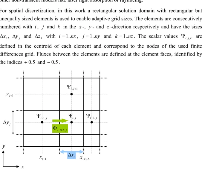
Finite differences are basically a method for calculating derivatives of discrete quantities. After dividing the variables into discrete intervals, derivatives of a general scalar can be approximated by the neighbouring values. The advantage to the competing finite element method is that no certain formulation of the equations to be solved is required and that the implementation as program code of lower complexity. The disadvantage is that finite differences work only on a structured and rectangular grid. Sub-grids and coordinate transformations can overcome these limitations only to a certain degree. In this work the structured rectangular grid is beneficial, because it allows an easy solver algorithm also for other non-transient models like laser light absorption or raytracing.

For spatial discretization, in this work a rectangular solution domain with rectangular but unequally sized elements is used to enable adaptive grid sizes. The elements are consecutively numbered with i, j and k in the x-, y- and z-direction respectively and have the sizes

i

x

Δ , Δy_j and Δz_k with i=1..nx, j =1..ny and k =1..nz. The scalar values Ψ_i,j,k are defined in the centroid of each element and correspond to the nodes of the used finite differences grid. Fluxes between the elements are defined at the element faces, identified by the indices +0.5 and −0.5.

Fig. 3-1: Sketch of an exemplary two-dimensional, noneqidistant, rectangular grid for finite differences discretization

y

x

j

i,

Ψ Ψ_i+1,j j

i−1,

Ψ

1 , +

Ψ_ij

i

x

Δ j

y

Δ

1

−

i

x

1

+

j

y

5 . 0

+

i

x

j

i−0.5,