Observational Research Using Propensity Scores
Karthik Raghunathan, J. Bradley Layton, Tetsu Ohnuma, and Andrew D. Shaw
In most observational studies, treatments or other “exposures” (in an epidemiologic sense) do not occur at random. Instead, treatments or other such interventions depend on several patient-related and patient-independent characteristics. Such factors, associated with the receipt vs nonreceipt of treatment, may also be—independently—associated with outcomes. Thus, con-founding exists making it difficult to ascertain the true association between treatments and outcomes. Propensity scores (PS) represent an intuitive set of approaches to reduce the influence of such “confounding” factors. PS is a computed probability of treatment, a value that is estimated for each patient in an observational study and then applied (in a variety of ways such as matching, stratification, weighting, etc.) to reduce distortion in the true nature of the association between treatment (or any similar exposure) and outcomes. Despite several advantages, PS-based methods cannot account for unmeasured confounding, ie, for factors that are not being included in the computation of PS.
Published by Elsevier Inc. on behalf of the National Kidney Foundation, Inc. Key Words:Propensity scores, RCTs
INTRODUCTION
Summarizing discussions at a“Roundtable on Value and Science-Driven Health Care,”authors noted the need for improvements in the conduct of randomized clinical tri-als (RCTs). They emphasized that large simple RCTs, that compare one treatment with another, can yield inter-nally valid results if conducted efficiently and effectively.1 Several other articles have also focused on strategies to improve RCTs.2This focus on RCTs, as the “gold stan-dard of clinical research”, comes from the fundamental assurance that RCTs provide—that outcomes are being compared across groups of patients that differ only in treatment (vs no treatment) and no other factors. In other words, patients’likelihood of treatment in an RCT is in-dependent of baseline attributes and determined by random assignment. Consequently, differences in out-comes are attributable to the differences in treatments. In observational settings, in contrast to RCTs, treatment is not randomly assigned and several patient-related and patient-independent attributes can influence the type of treatment received (or the receipt vs nonreceipt of treatment) and can also influence differences in out-comes independent of the differences in treatments. In other words, observational studies of health care inter-ventions are subject to confounding where systematic dif-ferences between groups of patients—that were treated vs not—result in difficulties in estimating the effects of treatment independent of all other factors.3 Propensity scores (PS) can be used to enable more accurate estima-tion of treatment effects in observaestima-tional studies (see Figs 1 and 2). In this article, we discuss how PS-based ap-proaches can be used to account for confounders in observational research and also discuss some limitations of PS-based methods.
PS WORK: A CONCEPTUAL SIMILARITY WITH RCTs PS-based methods offer an intuitive solution to the problem of confounding in observational research.4 By objectively quantifying a patient’s likelihood of receiving a particular treatment or exposure, based on measured baseline characteristics, ie, the PS value, re-searchers can construct “pseudo-populations,” where it is possible to estimate treatment effects more accu-rately. In these pseudo-populations, patients with
more similar likelihoods of treatment, ie, patients with similar baseline attributes (predisposition to treatment in routine clinical practice) differ in whether the treat-ment was actually received vs not. Thus, comparing outcomes, in pseudo-populations (chosen from the actual population), enables estimation of treatment ef-fects in ways that emulate the baseline “ exchange-ability” of treatment groups in RCTs. Populations of patients that were actually treated vs not treated are more comparable.
Consider an RCT designed to test a hypothesis using a simple 2-arm study design—patients could randomly receive treatment A or B (in a 1:1 ratio). For every patient randomly assigned to receive A, there is 1 patient randomly assigned to receive B. Outcomes can be directly compared because before the actual receipt of treatment A or B, each patient in the entire study sample had exactly the same probability of receiving A or B, completely independent of all other baseline characteris-tics. Chance alone determined whether a particular pa-tient received A or B. Because, in theory, the assigned treatment is the only systematic difference between groups, differences in outcomes (between groups) are presumed to be causally related to the differences in
actual treatments. In contrast to RCTs, in an
From the Department of Anesthesiology, Duke University Medical Center, Durham VA Medical Center, Durham, NC; Department of Epidemiology, Uni-versity of North Carolina at Chapel Hill, Chapel Hill, NC; and the Department of Anesthesiology, Vanderbilt University Medical Center, Nashville, TN.
IRB approval: This activity meets the VHA definition of“nonresearch.” Financial Disclosures: The authors declare that they have no relevantfi nan-cial interests.
Attribution of work: All authors made substantial contributions to concep-tion and design of this work, to the interpretaconcep-tion of data, to drafting or revising of the manuscript, and to thefinal approval of the version to be published and agree to be accountable for all aspects of the work. The work was performed at the Anesthesiology Service, Durham VA Medical Center. Durham, NC.
Address correspondence to Karthik Raghunathan, MD, MPH, Department of Anesthesiology, Duke University Medical Center/Durham VAMC, DUMC 3094, Durham, NC 27710. E-mail:[email protected]
Published by Elsevier Inc. on behalf of the National Kidney Foundation, Inc. 1548-5595/$36.00
observational study (of treatment A or B), without explicit randomization, direct comparisons of the out-comes are not feasible because several factors (indepen-dent of treatment) can contribute to the observed differences in outcomes. To address this problem, re-searchers can compute the PS. It is calculated as the probability of treatment, ie, the likelihood of treatment, conditional on observable characteristics.5Groups of pa-tients with similar calculated PS values have comparable likelihood of treatment but although some patients may actually receive treatment, others may not. Thus, we can compare patients with similar PS as they are “exchangeable.”
The PS is generally estimated using a multivariable model, typically logistic regression although other tech-niques may be used, with the exposure (ie, receipt vs nonreceipt of treatment) as the dichotomous dependent variable and with observable characteristics of patients as independent variables. The outcome itself should not be included in the PS model because treatment cannot “depend on”the outcome. Temporally, the outcome occurs after treatment. Once each
patient’s propensity or prob-ability for treatment is calcu-lated (value ranging from 0 to 1), it can be applied in a number of ways to minimize confounding. Rather than building a mathematical model purely predictive of treatment,6 the intent of PS models is to balance con-founders across treatment groups.7In other words, the goal of using PS is to ensure balance on all known con-founders across the groups
being compared. Known
risk factors for the outcome can be included as predictors to improve precision, but
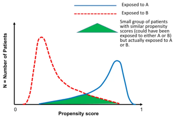
factors that are only predictive of the exposure (and unre-lated to the outcome, ie, instrumental variables) should not be included in the PS model—these factors are not con-founders as they are not independently related to the outcome.8 As a corollary, the purpose of “flipping a coin”in an RCT is to ensure that patients where the coin landed on one side are on average similar to patients where the coin landed on the other side. The purpose of the coin is not to “predict treatment”—it is to ensure exchangeability across treatment groups. PS estimates can also help determine whether comparisons (of groups with vs without treatment) are appropriate. To do this, re-searchers need to plot the distributions of PS scores in the treatment groups to see if treated and untreated groups show a considerable overlap in PS distributions or not
(see Figs 3 and 4). Comparisons are not appropriate if
patients are not in fact exchangeable, ie, if there is considerable nonoverlap. In the event of such large-scale nonoverlap of PS distributions, investigators need to
realize that patients who were actually treated vs not are too dissimilar in other ways than treatment alone. The op-tions here are to reconsider the choice of comparator or consider additional inclusion or exclusion criteria to arrive at a more exchangeability.
THE APPLICATION OF PS
A. Stratification: After estimation of PS, patients can be divided into several strata—quintiles, deciles, or more, depending on the size of the study. Each strata will have patients with very similar PS and that are, therefore, comparable on the distribution of baseline factors that predispose to treatment. However, in every stratum, only some patients are actually treated vs not treated and comparing within each stratum can, hence, estimate unconfounded treatment effects.9 These effects should be understood as minimally affected by confounding.9If there are differences in treatment effects across strata, this could imply either effect modification10 or the presence of unmeasured con-founding (particularly in the tails of the PS distri-bution).11 Effect modifi-cation means that the effects of treatment depend on the likelihood of treatment, a particular stratum of patients that is unlikely to be treated may only show small or no benefits of actual treatment while another stratum of patients that is highly likely to be treated may have signifi-cantly different benefits. If treatment effects are consistent across strata, researchers can collapse stratum-specific esti-mates into a single overall estimate. Conversely, if ef-fects vary across strata, investigators may consider reporting them separately or if the difference is likely because of bias, apply methods like trimming or matching to deemphasize the effect of the tails of the distribution.
B. Matching: Individuals with similar PS values that were actually treated vs not treated can be matched using various algorithms. In 1 common algorithm, “ pair-wise greedy matching without replacement,” each pa-tient with a given PS value who was treated is matched to another patient with an identical or nearly identical PS value (“greedy”in terms of how many decimal places are used to match PS values). The match is chosen from the group of patients who were not treated to create a pair and then both patients are removed from further matching. This approach creates groups with pairs of patients with the same PS distributions, and therefore, the same covariate distributions. In this CLINICAL SUMMARY
In most observational studies, treatments or other “exposures” do not occur at random. Rather, they “depend” on several patient-related and patient-independent characteristics that may also be related to outcomes. Hence, the effects of treatments on outcomes cannot be estimated without accounting for such “confounding.”
Propensity scores (PS) are probabilities of treatment and are computable for each patient in an observational study. These scores can be used in an intuitive set of approaches to reduce the influence of such confounding.
pseudo-population, confounding has been “broken” and outcomes can be directly compared like in an RCT where there is baseline exchangeability. The resulting risk estimate—difference in outcome between treated and untreated groups—is called the average effect of
treatment in the treated (ATT). This answers the ques-tion “what is the effect of treatment among patients who received the treatment vs those that did not.”There are a variety of other methods for matching (with replacement, closest neighbor, caliper matching etc.).
Observa onal study
Study Popula on of Pa ents with CKD observed to ini ate Sta n A or Sta n B
12 % 13%
Ini ators of A N= 2,000
Matching based on propensity scores used to match pa ents ini a ng A that are similar
pa ents ini a ng B.
Not all pa ents are similar – hence only 4000 pa ents of 10,000 are successfully matched. Baseline factors differ between two groups
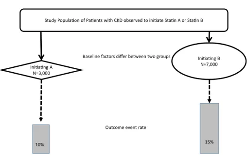
Ini a ng A N=3,000
Ini a ng B N=7,000
Ini ators of B N= 2,000
The extent to which an absolute 1% difference in the event rate -is affected by unmeasured baseline differences -is unclear. However, in the PS matched group of 4000 pa ents (2000 ini ators of A matched to 2000 ini ators of B), pa ents are comparable at baseline on all observable factors (that should
have been included in the computa on of PS).
Figure 2. Propensity scores used to create a matched cohort of patients that are comparable on baseline characteristics. Observa onal study
Study Popula on of Pa ents with CKD observed to ini ate Sta n A or Sta n B
Baseline factors differ between two groups
Outcome event rate
10% 15%
The extent to which outcome differences – an absolute 5% difference in the event rate – are affected by baseline differences is unclear. Mul variate regression analysis, with the outcome as the dependent variable and with baseline
covariates with treatment as predictors (independent variables) is commonly used. Ini a ng A
N=3,000
Ini a ng B N=7,000
Although the sample size can be reduced by matching, excluding patients who failed to match removes those without good exchangeability. Unmatched patients have no corresponding counterpart (patients that have similar PS but with opposite treatment assignment). However, in instances of poor PS overlap, the matched population may represent a very small, atypical pseudo-population that is not representative of the over-all population; if there is effect measure modification along the distribution of the PS, then the matched sam-ple may yield an effect measure estimate in only a small subset, which may differ from the overall population. C. Weighting: The PS can also be transformed into
weights and applied back to the original study popula-tion to create pseudo-populapopula-tions of treated and un-treated patients with similar PS distributions (and thus similar balance of covariate distributions). One type of weights, called standardized mortality ratio weights, or ATT weights, leaves the treated patients as is (ie, assigned weight ¼1), but “re-weights” the comparison group to have a similar PS distribution as the treated (weight ¼ PS/(1 2 PS)).12 The treatment
effect estimated in this weighted pseudo-population also yields the ATT (similar to the matching approach); however, all patients are retained in this analysis. Although there are no “unmatched” patients, out-comes are weighted down by untreated patients (with lower propensities). Another approach is to use inverse probability of treatment weights that are also estimated from the PS. When applying these weights to the population, the treated and comparison groups are weighted by the inverse of their actual exposure (treated weight ¼1/PS; comparator weight ¼1/(1 2 PS)). For practical purposes, weights can be stabilized by the marginal prevalence of exposure (Pe) to reduce
the influence of small group sizes (treated
weight ¼Pe/PS; comparator weight ¼(1 2 Pe)/(1 2 PS)). When these weights are applied, both treatment groups are weighted to the overall population, and hence, treatment effects that are estimated (in this in-verse probability of treatment weights-weighted pseudo-population) yield the average treatment effect. The question being answered here“what is the effect of treatment if the entire population were treated vs none of the population were treated?.”13This approach may not be appropriate in settings where individuals are unlikely to receive treatment (eg, comparing treatment with no treatment in a population without indications for treatment or with contraindications to treatment). Restriction of the comparison group to those with indi-cations for treatment or with an active comparator (eg, users of acceptable alternatives) may result in better comparisons.14
OTHER OPTIONS AND DEVELOPMENTS IN THE FIELD OF PS
There is considerable ongoing research on the estimation and application of PS in observational research. High-dimensional PS estimation is a tool developed for the auto-mated selection of large numbers of empirically identified potential covariates available in administrative health care databases,15potentially including hundreds of diagnoses, procedures, and medications that may be confounders or associated with confounders when researchers are trying to use observational data to estimate treatment effects. Another development, preference score, is a transforma-tion of the PS to study groups of patients with the greatest equipoise between strategies. By removing individuals very unlikely to be treated or very likely to be treated, the sample is restricted to, and the analysis performed only on, individuals with reasonable expectation of receiving vs not receiving treatment in the real world (ie, groups with PS values closer to 0.5 are identified and groups with PS values close to 0 or 1 are excluded).16
Disease risk scores (DRS) are similar to PS, in that they are composite scores of multiple covariates, but rather than modeling the likelihood of treatment, DRS model the likelihood of experiencing the outcome. DRS can be applied in similar matching strategies as PS, but they do not balance covariates between treatment groups like the PS do. Estimation of DRS can be more challenging than Propensity score
N = Number of Patients
0 1
Exposed to A
Exposed to B
Small group of paents with similar propensity scores (could have been exposed to either A or B) but actually exposed to A or B.
Figure 3. Propensity Density Plot: Propensity Scores (on the x-axis, range from 0-1) are plotted against the Number of Patients (on the y-axis). This figure shows few patients being matched.
Propensity score
N
0 1 Exposed to A
Exposed to B
Large group of paents with similar propensity scores (could have been exposed to either A or B) but actually exposed to A or B
the PS, but DRS may perform better in settings of PS non-overlap. DRS may be more stable over time because while treatment patterns can change (ie, propensity for treat-ment can change over time), the etiology of disease pro-cesses remains constant.17
THE EXAMPLE
Consider 2 hypothetical epidemiologic studies evaluating the effect of statins on changes in estimated glomerular filtration rates among patients with CKD: one investi-gating whether initiating a statin is more beneficial than not and another investigating the comparative effective-ness of 2 different statins. These 2 research questions are related, but they reflect 2 very different comparisons be-tween treatment groups. Although the statin vs no statin comparison considers new users and nonusers, the statin A vs statin B analysis compares 2 treatment groups which have both been evaluated by a physician and prescribed a statin: the confounders surround the choice of statin in the second example, but in thefirst, they surround the deci-sion about whether to treat.
In the statin new user (treatment initiator) vs nonuser study, the users are identified at initiation, and a relevant index date is selected to begin the comparison with pa-tients with CKD who are not receiving a statin. A PS model would be estimated, including relevant covariates measured before the index date, but statin nonusers may have clinical and behavioral characteristics which make them so different from the users of statins (eg, reduced ac-cess to health care, poor adherence, frailty, poor health habits, etc.) that confounding (and the risk for worse out-comes) may not be fully controllable.18-20 Distributions
and plots of PS values reflect this lack of
exchangeability21with a high likelihood of residual con-founding. PS matching would result in identification of only a small minority, while weighting may exaggerate treatment effects among atypical users. A more thought-fully identified comparison group (eg, initiators of another medication, or a more restricted, similar group of nonus-ers) may be warranted to avoid such residual confound-ing.14
In the comparative effectiveness analysis of 2 groups of patients (initiating statin A or statin B), identified at initi-ation of the mediciniti-ation, relevant baseline covariates measured before initiation can be used to obtain PS values and then to plot them, revealing good overlap.21 This is because both groups of patients met criteria for initiation of statins and only a few relevant factors deter-mined the choice of statin A vs B. Stratifying along the PS distribution would result in many strata with adequate numbers of patients receiving A or B for comparisons to be meaningful. Matching would exclude few patients and retain the vast majority. Comparisons in the pseudo-populations (created by stratification, matching, or weighting) should all yield estimates free of observable confounding.
Real-World Examples
PS methods have been widely used in clinical and epide-miologic research of kidney disease to control for
differ-ences between exposure groups. Various PS matching and weighting applications can be found in studies evalu-ating the safety22and effectiveness23of medications in kid-ney disease patients, evaluating the strength of risk factors in predicting kidney replacement therapy,24estimating the protective effect of medications against renal events,25 esti-mating the long-term effects of acute kidney injury,26and many others.
STRENGTHS
PS-based methods are useful in settings where outcomes are uncommon because covariates (used to mathemati-cally model treatment as the dependent variable) tend to be more prevalent, especially in observational settings with large numbers of covariates available in electronic medical records or administrative claims databases.4,27 Additionally, PS estimates yield treatment effects in defined subpopulations, so after stratification, matching, or weighting, the new pseudo-population’s covariate distributions can be plotted, the balance of covariates inspected, and the actual population on which inferences are being derived is known.
LIMITATIONS
Although PS methods allow for intuitive visualization of exchangeability between treatment groups, like in an RCT, and although PS-based methods yield estimates that are not confounded by measured factors (that were included in the PS model), unmeasured characteristics that are not captured in data or not included in the PS model will remain“unbalanced”and capable of causing confounding. Last, although PS methods can be used to guide the choice of a comparison group, application of these methods cannot compensate for fundamental study design flaws, such as improper choice of comparator, selection bias, measurement error, or missing data. Conceptually, an analogy may be made to civil prosecu-tions. To prove the effects of treatment by“a preponder-ance of the facts,” observational studies can only“build the case”using available evidence. Facts that are relevant, but that are not available to the prosecutor, can lead to wrongful convictions. After all, without random assign-ment, no observational study can truly be an“open and shut”case.
REFERENCES
1. Grossmann C, Sanders J, English RA. Rapporteurs. Institute of Medicine: Roundtable on Value and Science-Driven Health Care. Board on Health Care Policy. Forum on Drug Discovery, Deve-lopment, and Translation. National Academies Press (US); 2013. The National Academies Collection: Reports funded by National Institutes of Health.
2. Ioannidis JP. How to make more published research true.PLoS Med. 2014;11(10):e1001747.
3. Walker AM. Confounding by indication.Epidemiology. 1996;7(4):335-336.
4. Rubin DB. Estimating causal effects from large data sets using pro-pensity scores.Ann Intern Med.1997;127(8 Pt 2):757-763.
6. Westreich D, Cole SR, Funk MJ, Brookhart MA, Sturmer T. The role of the c-statistic in variable selection for propensity score models. Pharmacoepidemiol Drug Saf.2011;20(3):317-320.
7. Wyss R, Ellis AR, Brookhart MA, et al. The role of prediction modeling in propensity score estimation: an evaluation of logistic regression, bCART, and the covariate-balancing propensity score. Am J Epidemiol.2014;180(6):645-655.
8. Brookhart MA, Schneeweiss S, Rothman KJ, Glynn RJ, Avorn J, Sturmer T. Variable selection for propensity score models.Am J Epi-demiol.2006;163(12):1149-1156.
9. Rosenbaum PR, Rubin DB. Reducing bias in observational studies using subclassification on the propensity score. J Am Stat Assoc. 1984;79(387):516-524.
10. Sturmer T, Rothman KJ, Glynn RJ. Insights into different results from different causal contrasts in the presence of effect-measure modifi ca-tion.Pharmacoepidemiol Drug Saf.2006;15(10):698-709.
11. Sturmer T, Rothman KJ, Avorn J, Glynn RJ. Treatment effects in the presence of unmeasured confounding: dealing with observations in the tails of the propensity score distribution—a simulation study. Am J Epidemiol.2010;172(7):843-854.
12. Sato T, Matsuyama Y. Marginal structural models as a tool for stan-dardization.Epidemiology.2003;14(6):680-686.
13. Robins JM, Hernan MA, Brumback B. Marginal structural models and causal inference in epidemiology. Epidemiology. 2000;11(5):550-560.
14. Lund JL, Richardson DB, Sturmer T. The active comparator, new user study design in pharmacoepidemiology: historical foundations and contemporary application.Curr Epidemiol Rep.2015;2(4):221-228. 15. Schneeweiss S, Rassen JA, Glynn RJ, Avorn J, Mogun H, Brookhart MA. High-dimensional propensity score adjustment in studies of treatment effects using health care claims data. Epidemi-ology.2009;20(4):512-522.
16. Walker AM, Patrick AR, Lauer MS, et al. A tool for assessing the feasibility of comparative effectiveness research. Comp Eff Res. 2013;3:11-20.
17. Wyss R, Ellis AR, Brookhart MA, et al. Matching on the disease risk score in comparative effectiveness research of new treatments. Phar-macoepidemiol Drug Saf.2015;24(9):951-961.
18. Glynn RJ, Schneeweiss S, Wang PS, Levin R, Avorn J. Selective pre-scribing led to overestimation of the benefits of lipid-lowering drugs.J Clin Epidemiol.2006;59(8):819-828.
19. Brookhart MA, Patrick AR, Dormuth C, et al. Adherence to lipid-lowering therapy and the use of preventive health services: an investigation of the healthy user effect. Am J Epidemiol. 2007;166(3):348-354.
20. Dormuth CR, Patrick AR, Shrank WH, et al. Statin adherence and risk of accidents: a cautionary tale. Circulation. 2009;119(15): 2051-2057.
21. Layton JB, Brookhart MA, Jonsson Funk M, et al. Acute kidney injury in statin initiators. Pharmacoepidemiol Drug Saf. 2013;22(10):1061-1070.
22. Winkelmayer WC, Liu J, Setoguchi S, Choudhry NK. Effectiveness and safety of warfarin initiation in older hemodialysis patients with incident atrial fibrillation. Clin J Am Soc Nephrol. 2011;6(11):2662-2668.
23. Akizawa T, Tsubakihara Y, Hirakata H, et al. A prospective obser-vational study of early intervention with erythropoietin therapy and renal survival in non-dialysis chronic kidney disease patients with anemia: JET-STREAM Study. Clin Exp Nephrol. 2016;20(6): 885-895.
24. Ng DK, Moxey-Mims M, Warady BA, Furth SL, Munoz A. Racial~ differences in renal replacement therapy initiation among children with a nonglomerular cause of chronic kidney disease.Ann Epide-miol.2016;22(11):780-787.
25. Layton JB, Hansen MK, Jakobsen CJ, et al. Statin initiation and acute kidney injury following elective cardiovascular surgery: a popula-tion cohort study in Denmark. Eur J Cardiothorac Surg. 2016;49(3):995-1000.
26. Hansen MK, Gammelager H, Jacobsen CJ, Hjortdal VE. Acute kid-ney injury and long-term risk of cardiovascular events after cardiac surgery: a population-based cohort study.J Cardiothorac Vasc Anesth. 2015;29(3):617-625.