Spatial aspets of two-photon entanglement,
diration, and sattering
Publisher: Casimir Research School, Lorentzweg 1, 2628 CJ Delft, The Netherlands.
ISBN: 97890 8593 089-1
Print: Gildeprint Drukkerijen - The Netherlands
Cover Design: Martijn van Leipsig
Spatial aspets of two-photon entanglement,
diration, and sattering
PROEFSCHRIFT
ter verkrijging van
de graad van doctor aan de Universiteit Leiden,
op gezag van rector magnificus prof. mr. P. F. van der Heijden,
volgens besluit van het College voor Promoties
te verdedigen op dinsdag 21 december 2010
klokke 13:45 uur
door
Wouter Herman Peeters
Promotor: Prof. dr. J. P. Woerdman Universiteit Leiden Copromotor Dr. M. P. van Exter Universiteit Leiden Leden: Prof. dr. C. W. J. Beenakker Universiteit Leiden Dr. M. J. A. de Dood Universiteit Leiden
Prof. dr. A. Lagendijk Universiteit van Amsterdam (UvA) en Universiteit Twente
Prof. dr. G. Nienhuis Universiteit Leiden Prof. dr. J. M. van Ruitenbeek Universiteit Leiden Prof. dr. J. P. Torres Universitat Polit`ecnica
de Catalunya (UPC)
Dr. V. Zwiller Technische Universiteit Delft
Paranimfen: ir. R. van Melle en drs. O. A. Tuinenburg
The research described in this thesis is part of the research programme of the Foundation for Fundamental Research on Matter (FOM), which is part of the
Netherlands Organisation for Scientific Research (NWO).
The research has been carried out at the
Quantum Optics and Quantum Information group, which is part of the Leiden Institute of Physics (LION) of the Faculty of Science of Leiden University.
Additionally, the academic environment has been supported by the Casimir Research School, which is supported by LION at Leiden University and
the Kavli Institute of Nanoscience at Delft University of Technology.
An electronic version of this dissertation is available at the Leiden University Repos-itory (https://openaccess.leidenuniv.nl).
1 Introduction 1
1.1 Interference in optics . . . 1
1.1.1 Young’s experiment: interference of waves . . . 1
1.1.2 One-photon and two-photon interference . . . 2
1.1.3 Spontaneous parametric down-conversion: a source of pairs of entangled photons . . . 4
1.2 Research topics in this theses . . . 5
1.2.1 Two-photon interference: three themes . . . 5
1.2.2 Theme 1: Orbital angular momentum entanglement . . . 5
1.2.3 Theme 2: Two-photon diffraction from a double slit . . . 6
1.2.4 Theme 3: Two-photon scattering . . . 8
1.3 Quantum description of SPDC light . . . 9
1.3.1 Motivation . . . 9
1.3.2 Two approaches to describe SPDC light . . . 9
1.3.3 Two-photon field . . . 10
1.3.4 Expression for the two-photon field . . . 12
1.3.5 Klyshko picture . . . 13
1.4 Thesis outline . . . 14
2 Orbital angular momentum analysis of high-dimensional entangle-ment 17 2.1 Introduction . . . 18
2.2 Continuous two-photon amplitude . . . 19
2.2.1 Generated two-photon amplitude . . . 19
2.2.2 Interference after image rotation . . . 20
2.3 Discrete modal analysis . . . 24
2.3.1 Schmidt decomposition of the detected two-photon amplitude 24 2.3.2 Modal decomposition and the Schmidt number . . . 27
2.3.3 The physical significance ofV(θ) . . . 28
2.4 Experimental results . . . 29
2.4.2 Spiral phase plate . . . 32
2.4.3 Alignment . . . 33
2.4.4 Experimental results for detection through circular apertures 34 2.4.5 Experimental results forl= 1 detection . . . 38
2.5 Concluding discussion . . . 40
2.6 Acknowledgements . . . 41
3 Optical characterization of periodically poled crystals 43 3.1 Introduction . . . 44
3.2 Phase matching in a periodically poled crystal . . . 45
3.3 Experimental apparatuses . . . 47
3.4 Experimental results . . . 51
3.4.1 Maker fringes in angular intensity pattern of SPDC light . . . 51
3.4.2 Maker fringes in spectrum of SPDC light . . . 55
3.4.3 Maker fringes in temperature dependence of SHG . . . 55
3.5 Interpretation of Maker fringes in terms of poling quality . . . 57
3.5.1 Fourier analysis of small and slowly varying deformations of the poling structure . . . 57
3.5.2 Analysis of Maker fringes in terms of poling quality . . . 61
3.6 Conclusions . . . 63
3.7 Acknowledgements . . . 64
4 Engineering of two-photon spatial quantum correlations behind a double slit 65 4.1 Introduction . . . 66
4.2 Theory: Two-photon state engineering . . . 68
4.2.1 Electromagnetic field behind double slit . . . 68
4.2.2 Quantum state engineering . . . 69
4.2.3 Incident two-photon state . . . 71
4.2.4 Near-field imaging scheme . . . 73
4.2.5 Far-field imaging scheme . . . 75
4.3 Theory: Interference behind the double slit . . . 76
4.3.1 State determination by two-photon interference . . . 76
4.3.2 Interpretation of the two-qubit Bloch sphere . . . 78
4.3.3 One-photon interference . . . 79
4.3.4 Duality between unconditional one-photon interference and two-photon interference . . . 80
4.4 Experimental apparatus . . . 81
4.4.1 General information . . . 81
4.4.2 Experimental apparatus in front of double slit . . . 81
4.4.3 Experimental apparatus behind double slit . . . 83
4.5 Experimental results . . . 85
4.5.2 Analysis and tuning of two-photon interference patterns . . . 85
4.5.3 Near-field imaging atϕ= 0 . . . 88
4.5.4 Far-field imaging atϕ= 0 . . . 89
4.5.5 Near-field imaging at nonzero curvature phase . . . 91
4.5.6 Far-field imaging at nonzero curvature phase . . . 92
4.6 Conclusion . . . 93
4.7 Discussion: tuning in high-dimensional Hilbert space . . . 94
4.8 Acknowledgements . . . 95
4.9 APPENDIX: Validity of the model for various phase-matching ge-ometries . . . 95
5 Observation of two-photon speckle patterns 99 5.1 Introduction . . . 100
5.2 Theory . . . 100
5.3 Experimental setup . . . 103
5.4 Experimental results . . . 105
5.5 Discussion . . . 106
5.6 Conclusion . . . 107
5.7 Acknowledgements . . . 107
5.8 APPENDIX: Derivation of the two-photon speckle autocorrelation function . . . 107
6 Spatial pairing and antipairing of photons in random media 111 6.1 Introduction . . . 112
6.2 Random unitary scattering of labeled photons . . . 112
6.3 Experiments . . . 116
6.3.1 Experimental scheme . . . 116
6.3.2 Details of experimental apparatus . . . 118
6.3.3 Experimental results . . . 120
6.4 Concluding discussion . . . 123
6.5 Outlook . . . 124
6.6 Acknowledgements . . . 125
6.7 APPENDIX: Scattered density matrix . . . 125
Bibliography 129
List of publications 139
Nederlandse samenvatting 141
Nawoord 147
1
Introdution
1.1 Interference in optics
1.1.1 Young’s experiment: interference of waves
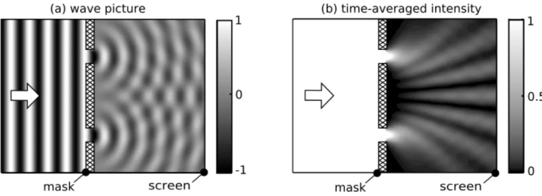
Around 1801, the British scientist Thomas Young demonstrated that light prop-agates like a wave. Light waves, in contrast to light rays, can form interference patterns. Young illuminated a mask with two parallel slits with monochromatic spatially coherent light and projected the transmitted light onto a screen. He ob-served a periodic intensity pattern of bright and dark lines, which he explained as an interference pattern. Figure 1.1 illustrates a simulation of a wave passing through a mask with two slits. The two waves that emerge from the slits expand in a circular manner such that they cross each others path. In the low-intensity regions, the phases of the two waves are opposite, and the waves interfere destructively at any instant of time. In the high-intensity regions, both waves interfere constructively yielding a larger detected intensity.
Figure 1.1: (a) Simulation of a wave propagating through a mask with two slits. The grey scale represents the wave displacement at some instant of time. (b) An interference pattern is formed in the time-averaged intensity profile behind the mask. Around 1801, Thomas Young demonstrated that light produces such intensity pattern. He visualized this interference pattern by projecting the transmitted light onto a screen.
1.1.2 One-photon and two-photon interference
The quantum theory of light describes the quantum state|Ψiof the electromagnetic field [3,4]. Formally, this theory is obtained by applying a procedure called canonical quantization to the classical theory of the electromagnetic field. The foundation of multiphoton interference within quantum optics was laid by Glauber in 1963 in his influential work on quantum optical coherence [5]. The quantum theory replicates the occurrence of the classical interference patterns of the intensity similar to the one shown in Fig. 1.1(b). Additionally, Glauber’s analysis makes clear that quantum interference can occur inn-fold intensity correlations betweennseparate detectors. This type of optical interference is now referred to asn-photon interference.
Young’s classical interference pattern in Fig. 1.1 is a one-photon interference phenomenon. One-photon interference refers to a structure in the photon detection rate in a single detector. The photon detection rate is [5]
R(1)(r, t)∝ hΨ|Eˆ−(r, t) ˆE+(r, t)|Ψi, (1.1) where ˆE±(r, t) are the positive and negative frequency electric-field operators at
positionrand timet. A one-photon interference pattern can in principle be formed by a single photon only. So if one would perform Young’s experiment with a single photon, the probability of where the photon can be absorbed corresponds to the intensity pattern obtained from the classical wave theory [see Fig.1.1(b)].
two detectors. Glauber argued that this coincidence rate is [5]
R(2)(r1, t1;r2, t2)∝ hΨ|Eˆ−(r1, t1) ˆE−(r2, t2) ˆE+(r2, t2) ˆE+(r1, t1)|Ψi, (1.2)
wherer1,2andt1,2are space and time coordinates of the two detectors. It may not
be obvious from Eq. (1.2) how two-photon interference can occur. Let us therefore construct the two-photon state∗
|Ψi= √1 2
Z
dk1dk2φ(2)(k1,k2)ˆa†(k1)ˆa†(k2)|vaci, (1.3)
whereφ(2)(k
1,k2) =φ(2)(k2,k1) without loss of generality,|vaciis the
continuous-mode vacuum, and ˆa†(k) is the continuous-mode photon creation operator with
momentumk. For our interest in simplicity, we have restricted ourselves to one po-larization only. Let us also specialize to paraxial light whereφ(2)(k
1,k2) is nonzero
only fork vectors that are oriented paraxially. By combining Eqs. (1.2) and (1.3), we find the two-photon interference pattern†
R(2)(r1, t1;r2, t2) ∝ Z
dk1dk2 φ(2)(k1,k2) exp (ik1·r1−i|k1|ct1)
×exp (ik2·r2−i|k2|ct2) 2 , (1.4)
where c is the speed of light. The absolute square operation directly reveals the interference mechanism behind two-photon interference. The expression between |..|2 is the two-photon wave packet, which is a complex (rotating) amplitude as a
function of two coordinates. Each coordinate is propagated according to the scalar wave equation of light.
Two-photon interference is especially interesting if the two photons in Eq. (1.3) are entangled. In the entangled case, the two-photon amplitude does not factorize in two functions‡, i.e.,
φ(2)(k1,k2)6=f(k1)f(k2).
∗ We use the continuous-mode formalism with usual commutation relations and field op-erators given by Eqs. (10.10-1)-(10.10-4) in Ref. [3]. Normalization then corresponds to
R
dk1dk2|φ(2)(k1,k2)|2 = 1, where we have imposed φ(2)(k1,k2) = φ(2)(k2,k1) without
loss of generality since any asymmetry drops out of Eq. (1.3).
† We adjusted the electric-field operator in Eq. (1.2) to a similar operator related to the square root of the photon density (the continuous-mode version of equation (12.3-1) in Ref. [3]). The expression for this adjusted field operator (in single-polarization form) is ˆV+(r, t) =
p
(2π)−3R
dkˆa(k) exp[ik·r−i|k|ct].
‡ It is debatable whether inseparability also implies entanglement. For example: is it correct to callφ(2)(k
1,k2) =f(k1)g(k2) +f(k2)g(k1) entangled? We will refer to this two-mode form
Figure 1.2: Experimental geometry for the operation of spontaneous parametric down-conversion. The down-converted light is spatially multimode (indicated by the arrows). Each down-converted photon pair is spatially entangled due to conservation of transverse momentum in the down-conversion process.
If this function would factorize, the two-photon interference pattern would become a trivial multiplication of the one-photon interference patterns, i.e.,
R(2)(r1, t1;r2, t2)∝R(1)(r1, t1)R(1)(r2, t2) [ifφ(2)(k1,k2) factorizes].
If the two-photon amplitude does not factorize, the one-photon interference pattern generally gets washed out, but, at the same time, the two-photon interference pat-tern retains its high visibility. Two-photon interference occurs most prominently in a two-photon state. The presence of a three-photon component (or more pho-tons) will lower the visibility of the two-photon interference pattern ifφ(2)(k
1,k2)
is not factorizable. Therefore, one requires two-photon states to study interesting two-photon interference phenomena with high visibility.
1.1.3 Spontaneous parametric down-conversion: a source of pairs of entangled photons
Nowadays, two-photon interference experiments are commonly performed with pho-ton pairs produced by the nonlinearχ(2) process of spontaneous parametric
Figure 1.3: Generic scheme of the two-photon interference experiments discussed in this thesis. Two-photon interference phenomena are experimentally observed via the coincidence count rate in the plane of the detectors.
interference. Two-photon interference was first observed in 1987 by Ghosh, Hong, Ou, and Mandel [7, 8].
1.2 Research topics in this theses
1.2.1 Two-photon interference: three themes
The research in this thesis addresses spatial aspects of two-photon interference. The work is mainly experimental although our experiments are supported by theoretical models. The research can be divided into three research themes: We address (1) orbital angular momentum entanglement, (2) two-photon diffraction from a double slit, and (3) two-photon scattering of a random medium.
Despite their diversity, all themes are strongly related to one another. This is because two-photon interference and spatial entanglement play dominant roles in all themes. A generic scheme of all interference experiments is displayed in Fig. 1.3. Pairs of spatially entangled photons are emitted by the SPDC source and propa-gate through the experimental setup before being detected by two single-photon detectors. The propagation part is different for each experiment depending on the addressed research theme. Figure 1.4 illustrates the three setups that correspond to the three research themes. These research themes are discussed below in Secs. 1.2.2-1.2.4.
1.2.2 Theme 1: Orbital angular momentum entanglement
must collapse into a spatial profile with −~l. This is because the pump beam is
just a Gaussianl= 0 beam, and OAM is conserved in the down-conversion process. The quantum state of the photon pair can thus be tentatively written as∗
|Ψi ∼
∞
X
l=−∞
p
Pl +l~
1⊗
−l~
2 [omitting radial properties],
where the probabilities Pl = P−l correspond to the distribution over the orbital angular momentum spectrum.
The distribution of thePlcoefficients can, in principle, be determined from the incoherent OAM distribution of just one of the photons [20, 21]. Such a measure-ment does, however, not depend on whether the photons are really entangled or not. The photons could equally well be a pair of independent incoherent photons with some OAM spectrum. In the literature, it was argued that the OAM distribution could also be determined via two-photon interference involvingboth entangled pho-tons [22]. The experimental technique for this experiment is illustrated in Fig. 1.4 (theme 1). The orbital-angular momentum spectrum is contained in the visibility of the multimode Hong-Ou-Mandel dip as a function of the rotation angle of the image rotator [22]. In this thesis, we have used this challenging technique to determine the OAM distribution of the entangled photons. We also consider several special cases and provide a more detailed theoretical analysis supporting the experiment.
1.2.3 Theme 2: Two-photon diffraction from a double slit
Starting from 1994, a lot of experiments have addressed two-photon diffraction from a double-slit [23–35]. So why would one still want to study this topic? The reason is that the diversity of possible two-photon interference patterns behind a double slit has, we believe, not been widely appreciated. In fact, most of the possible forms of spatial entanglement behind the double slit have remained unexplored so far.
The most general two-photon state behind the double-slit (under symmetric two-photon illumination) can be written as
|Ψi= cos (α/2)
|↑↓i√+|↓↑i 2
+eiϕsin (α/2)
|↑↑i√+|↓↓i 2
, (1.5)
where | ↑i and | ↓i represent transmissions through the top and bottom slit, and parametersαandϕdetermine the quantum state. This state can be recognized as a superposition of two maximally entangled Bell states. The first Bell state cor-responds to photons going through opposite slits; the second term corcor-responds to
∗ The full Schmidt decomposition also involves the radial properties of the mode profiles (see
Ref. [9] and chapter 2): |Ψi= P∞
l=−∞ ∞
P
p=0
p
photons choosing the same slit. So far, no attention has been paid to the experi-mental tuning of the phase ϕ. However, this phase is extremely important for the degree and type of entanglement. One could, for example, consider the maximally entangled state at α=ϕ= 12π. In this form of entanglement, the path of photon 1 is quantum correlated with the state | ↑i ±i| ↓i of photon 2, while path-path correlation is absent.
In comparison to other experiments on the two-photon double slit, our research is novel in three different ways. First, we demonstrate how to engineer the spatial entanglement with full control over state parametersαandϕ. Secondly, our anal-ysis provides a deeper understanding of the spatial structure in the entanglement between down-converted photons. We address, for the first time, phase-sensitive aspects of the two-photon field in the near-field of the generating crystal. Finally, we measure entire two-photon diffraction patterns in the far-field of the double slit with unprecedented quality. Our experiments reveal, in a very pure manner (namely: double-slit diffraction), the large diversity of two-photon interference pat-terns.
1.2.4 Theme 3: Two-photon scattering
This theme is the most advanced. Until now, the propagation of entangled photon pairs through a random medium has never been investigated experimentally. Only recently, a few theoretical papers have appeared [36–38]. Why would one want to study such a topic? The reason is simple. One-photon interference effects in ran-dom media are widely studied and have proven to be extremely interesting and di-verse [39, 40]. Interesting phenomena within one-photon scattering are speckle [41], enhanced backscattering [42, 43], universal conductance fluctuations [44], and An-derson localization of light [43, 45–47]. Can we discover similar phenomena for two-photon interference in the case of two-photon scattering?
1.3 Quantum description of SPDC light
1.3.1 Motivation
In the previous section, we presented an overview of the topics that are investigated in this thesis. Despite the diversity, all experiments address the same observable: the time-averaged coincidence count rate in continuous-wave (cw) pumped, low-gain∗
SPDC light. For each experiment, we have made a theoretical model providing a solid understanding of the experimental results. All models are based on a quantum description of SPDC light. More specifically, the models are based on a single concept called the two-photon field. As the two-photon field plays a central role in this thesis, we have devoted Secs. 1.3.2-1.3.5 to a discussion of the theoretical foundation of this concept.
1.3.2 Two approaches to describe SPDC light
The description of SPDC light requires a quantum-mechanical treatment of the SPDC process†. There is a substantial amount of literature on the theory of
SPDC [3,4,49,51–65]. The treatments can be divided into two categories depending on the approach.
The first approach uses the quantized version of the input-output relations of a parametric amplifier [3, 4, 49, 60–62, 64]. The light in the output channels is de-scribed as a noisy signals exhibiting quantum Gaussian noise [49,58]. This approach is suitable for both the low-gain and high-gain regime of SPDC and has gained pop-ularity in the last decade [50, 60, 62, 64, 66]. Most papers just analyse a two-channel parametric amplifier (signal and idler), although spatially multimode SPDC has also been treated in this way [60, 61, 67].
The second approach is based on a first-order perturbative analysis of the time-evolution operator [3, 51, 53–55, 57, 59, 63, 65, 68]. This approach only works in the low-gain regime since a first-order perturbation analysis yields at most a single pho-ton pair. All spatial and temporal correlations between the phopho-tons are contained in the resulting quantum state. As all experiments in this thesis are performed in
∗ Parametric gain corresponds to the strength at which the signal and idler fields are amplified due to parametric interaction with the strong pump beam. Low gain means that a generated photon pair has low probability (≪ 1) to stimulate the generation of another pair (thus creating four photons) during transmission through the crystal.
† Otherχ(2)processes like second harmonic generation and sum/difference frequency generation
the low-gain regime, we use a description of the SPDC light that is based on the perturbative approach (see Sec. 1.3.3).
1.3.3 Two-photon field
Based on the perturbative approach, the concept of the two-photon field was put forward in Refs. [54, 56] by Rubin, Klyshko, Shih, and Sergienko. In the first-order perturbation method, the quantum state of the generated SPDC light is calculated as [3, 53–55, 59, 65, 68]
|Ψ(τ)i ≈ |vaci −~i τ
Z
0
dt HIˆ (t)|vac,i (1.6)
whereτis the interaction time, and ˆHI(t) is the interaction Hamiltonian of theχ(2)
nonlinear process driven by a classical, paraxial, and monochromatic pump beam E(r, t) [3, 53, 59]. The interaction Hamiltonian contains two photon creation oper-ators and depends linearly on the driving field of the pump beam, the interaction volume, and the second-order nonlinear susceptibilityχ(2) of the crystal.
The second term in Eq. (1.6) is a two-photon component. The norm of this component grows linearly with the interaction time∗. Intuitively, state |Ψ(τ)i is
only experimentally meaningful if the norm of the two-photon component stays way below unity even for interaction times τ much greater than the transmission time through the crystal (which implies the low-gain regime). Then, the interaction time for which this norm equals unity corresponds to the average time between successive down-conversions†. The quantum state |Ψ(τ)i contains all spatial and
temporal correlations between the down-converted photons and is thus effective in describing multimode two-photon interference experiments [51, 68, 69].
The normalization of |Ψ(τ)i breaks down dramatically for large interaction times [3]. Nonetheless, this normalization issue is often ignored in the literature; in many papers, the interaction time is simply taken to infinite yielding [54,57,59,63,68]
|Ψ∞i ≡ |vaci −
i
~
∞
Z
−∞
dtHIˆ (t)|vaci. (1.7)
The normalizability of|Ψ∞ibreaks down on account of the first-order perturbation
method, the infinite interaction time, and the infinite duration of the driving cw pump beam (thus hΨ∞|Ψ∞i = ∞). Quite remarkably, this normalization issue is hardly ever discussed; it is, to the best of our knowledge, only addressed by
Shapiroet al. in Refs. [50, 62]. Mathematically, the state|Ψ∞i contains only two photons. In the laboratory, however, a typical SPDC source produces millions of photon pairs per second.
The two-photon field is defined as [54, 56]
A(x1, t1,x2, t2;z)≡ hvac|Eˆ+(x2, t2;z) ˆE+(x1, t1;z)|Ψ∞i, (1.8)
where ˆE+(x, t;z) is the positive frequency electric-field operator at transverse
posi-tionx, timet, and longitudinal positionz. In the paraxial and narrow-band regime (∆ω≪ω), the electric field operators can be expressed∗in units ofp
photons/m2s.
The two-photon field then acquires units (m2s)−1. The divergence of
|Ψ∞iis also present in the two-photon field in a sense that it is not square integrable over all positionsx1,2 and timest1,2. The reason is that the two-photon field stretches out
over an infinite amount of time. Nevertheless, its square amplitude in the time domain is finite and relates to the photon flux [54, 55, 62]. The two-photon field should thus be regarded as an unnormalizable two-photon wave packet† for which
its amplitude in the time domain is related to the photon flux.
Based on Refs. [54, 56], the time-averaged coincidence count rate between two detectors at transverse positionsx1andx2 becomes
Rcc(x1,x2;z)∝
1 2×
Z
A1
d2x′1 Z
A2
d2x′2 +1
2τg
Z
−1 2τg
dt′
A(x1+x
′
1, t,x2+x′2, t+t′;z) 2
, (1.9)
whereA1,2 are the transverse integration areas of the two detectors andτg is the
gating time window of the coincidence logic. In typical experiments, the gate time τg is much larger than the spread in arrival times of the photons. Therefore, the integral overdt′can be taken over an infinite interval without changing the outcome
of the integral. The factor 1
2 between parentheses applies to type-I SPDC and is
absent in type-II SPDC. This is because in type-I SPDC, the electric field operators in Eq. (1.8) have the same polarization and senseboth photons in the two-photon state. In type-II SPDC, the electric field operators in Eq. (1.8) are assumed to have orthogonal polarizations and individually address only one of the photons, which are now distinguishable instead of indistinguishable. The square absolute value operation in Eq. (1.9) directly reveals the two-photon interference mechanism.
∗ The expression for the electric-field operator in units of square-root photon flux is ˆE+(r, t) =
p
c/(2π)3R
dkaˆ(k) exp[ik·r−i|k|ct].
† For type-I SPDC, the identification with the symmetrized paraxial two-photon amplitude φ(2)(k1,k2) in Eq. (1.3) becomes:
A(r1, t1,r2, t2) = c
√
2 (2π)3
R
Spatial propagation of the two-photon field fromz= 0 toz=zd is described by applying the Maxwell electric-field propagators to each of the electric-field operators in Eq. (1.8). Naturally, spatial propagation is written down after a temporal Fourier transform, i.e,
A(x1, ω1,x2, ω2;zd) = Z
d2x′
1d2x′2h(x1, zd,x′1,0;ω1)h(x2, zd,x′2,0;ω2)
×A(x′
1, ω1,x′2, ω2; 0), (1.10)
whereh(xf, zf,xi, zi;ω) is the electric field propagator for any forward-propagating frequency-conserving optical system (see for example Ref. [70]). In principle, with the tools presented in this section, one can describe any low-gain two-photon inter-ference experiment in the form of Fig. 1.3.
The absence of an equality sign in Eq. (1.9) is rather unfortunate. Although Rubinet al.[54,56] actually use an equality sign there, they state that their equation “defines” rather than calculates the coincidence count rate [54]. From our point of view, an analysis of the relationship between the photon flux and the unnormalizable two-photon state |Ψ∞i is not clearly present in the literature∗. We conjecture,
however, that the proportionality sign can be replaced by an equality sign (assuming high detection efficiency). Our argument is that if one would plug in a normalized paraxial two-photon state in Eq. (1.8), one would precisely get a single coincidence count when integrating 1
2×
|A(x1, t1,x2, t2;z)|2 over coordinates x1,2 and t1,2.
The norm of |Ψ(τ)i in Eq. (1.6) can be interpreted as the expected number of photon down-conversions and grows linearly with interaction time τ. Therefore, it seems reasonable to assume that the proportionality sign in Eq. (1.9) can be replaced by an equality sign.
1.3.4 Expression for the two-photon field
Based on the treatments in Refs. [51, 69], and assuming the crystal to be infinitely wide in both transverse directions, the Fourier-transformed two-photon field of Eq. (1.8) is
A(q1, ω1,q2, ω2; 0) ∝ δ[ωp−(ω1+ω2)]Ep(q1+q2;z= 0)
×sinc
L
2∆kz(q1, ω1,q2, ω2)
, (1.11)
where δ(ω) is the Dirac-delta function, sinc(x) ≡ sin(x)/x, q1,2 are transverse
momenta of the two-photon field, ωp is the angular frequency of the pump beam, Lis the crystal length, andEp(q;z= 0) is the complex amplitude of the cw pump
beam in momentum representation (in the crystal-center plane). The function
∆kz(q1, ω1,q2, ω2)≡kz(q1+q2, ωp)−kz(q1, ω1)−kz(q2, ω2), (1.12)
is the wave vector mismatch along thezdirection of the crystal. Here,kz(q, ω) is the zcomponent of the wave vector of a plane wave inside the crystal with transverse momentumqand angular frequencyω. The proportionality in Eq. (1.11) contains a linear dependence on the effective nonlinearity and the length of the crystal. The two-photon field in Eq. (1.11) contains all you need to know to describe spatial and temporal effects in two-photon interference experiments. It is also very general as it applies to all cw-pumped, low-gain SPDC processes in any kind of phase-matching geometry: type-I (same polarization), type-II (different polarizations), and quasi phase matching∗.
Let us discuss some properties of the generated two-photon field in Eq. (1.11). First, the delta functionδ[ωp−(ω1+ω2)] ensures conservation of energy of the
down-converted photons. The delta function also demonstrates that the two-photon field is unnormalizable since it spreads out infinitely long in the time domain. Secondly, the spread in the total transverse momentum of the down-converted photon pair is limited by the spread in momentum of the incident beamE(q1+q2). Third,
the phase-matching condition in Eq. (1.12) limits the spread along the (q1−q2)
and (ω1−ω2) coordinates. The spread in the arrival time difference between the
two down-converted photons is inversely proportional to the phase-matching band-width, i.e., the spread in the (ω1−ω2) coordinate. For type-I phase matching, the
symmetry of the two-photon field under sign reversal of (ω1−ω2) implies that the
average arrival time difference between the photons is zero. Finally, and maybe most importantly, the two photons are entangled because Eq. (1.11) does not factorize into two functions of the individual coordinates.
1.3.5 Klyshko picture
The Klyshko picture provides a very intuitive interpretation of spatial correlations between down-converted photons [48, 52, 71]. This interpretation follows one de-tected photon at x1 backwards in time to the generating crystal where is is
con-verted into the second forward propagating photon via a virtual reflection at the (possibly curved) pump beam profile. The spatial profile of the coincidence rate Rcc(x1,x2) is now given by how well the two detectors “see each other” via this
reflecting path. The Klyshko picture is very convenient in use and will often provide a good first guess of what can be expected in two-photon coincidence experiments.
Nevertheless, the Klyshko picture has severe limitations as it does not involve aspects of phase matching. The phase-matching condition generally confines the angular spread of down-converted light and causes spectral and spatial aspects of the two-photon field to be correlated. The two-photon field in Eq. (1.11) can be adapted to a Klyshko-picture form by simply removing the sinc-function part, i.e.,
A(q1, ω1,q2, ω2; 0)∼δ[ωp−(ω1+ω2)]Ep(q1+q2;z= 0) [Klyshko picture].
The Klyshko picture works well in the thin-crystal limit whereL→0 in Eq. (1.11). Phase-matching aspects are very important in this thesis. Therefore, the Klyshko picture is generally insufficient to understand our experimental results. In chapter 4, we utilize near-field aspects of the two-photon field, which result from the phase-matching condition. In chapter 5, the phase-matching condition limits the dimensionality of the entanglement and the size of the two-photon speckle spots. In chapter 6, we use type-II down-conversion where the allowed optical detection bandwidth is drastically reduced by the phase-matching condition as compared to type-I phase matching. Chapter 3 is entirely devoted to a detailed investigation of the phase-matching condition in our crystals.
1.4 Thesis outline
This thesis contains four published papers (chapters 2-5) and one yet unpublished work (chapter 6) on two-photon interference. All works can be read independently. You might wish to read only a few of them. Below, we have provided a catchy description of each chapter to facilitate your choice.
• Chapter 2: It is well known that light can carry orbital angular momentum. The down-converted photons in SPDC light are entangled via their orbital angular momentum. If one of the photons is detected with orbital angular momentum +l~then the other collapses into −l~since the total amount of
• Chapter 3: This chapter contains a thorough characterization of SPDC and second harmonic generation (SHG) in periodically poled KTiOPO4. The investigated spatial aspects of the phase-matching condition
are essential for the two-photon field used in chapters 4-6. As a bonus, we dis-covered how the observed phase-matching rings in SPDC light contain quan-titative information on the quality of the poling structure in the nonlinear crystal.
• Chapter 4: Finally, more than 200 years after Young’s double-slit experi-ment, we present a complete and comprehensive description of the double-slit experiment for the two-photon case. Two-photon interfer-ence allows for a wide variety of different fringe patterns. We are the first to measure them all and with unprecedented quality (see cover of printed thesis). Our results are backed-up by our simple comprehensive model for two-photon double-slit fringe patterns. Special attention is paid to the two-photon phase front, an important aspect that has often been overlooked. To generate these patterns, we utilize phase-sensitive properties of the two-photon field in both the near-field and far-field of the non-linear crystal.
• Chapter 5: Wave propagation in random media has intrigued and occupied many physicists in the last five decades. The most prominent feature of a multiply scattered wave is its random interference pattern called speckle. We wondered what two-photon speckle patters with spatial entanglement would look like. In chapter 5 we present the first observation of two-photon speckle patterns. We have found out how the spatial structure within two-photon speckle patterns is related to the structure of the scattering medium. Spatial entanglement gives two-photon speckle a much richer structure than ordinary one-photon speckle.
2
Orbital angular momentum
analysis of high-dimensional
entanglement
We describe a simple experiment that is ideally suited to analyze the high-dimensional entanglement contained in the orbital angular momenta (OAM) of en-tangled photon pairs. For this purpose we use a two-photon interferometer with a built-in image rotator and measure the two-photon visibility versus rotation angle. Mode selection with apertures allows one to tune the dimensionality of the entan-glement; mode selection with spiral phase plates and fibers allows detection of a single OAM mode. The experiment is analyzed in two different ways: either via the continuous two-photon amplitude function or via a discrete modal (Schmidt) decomposition of this function. The latter approach proves to be very fruitful, as it provides a complete characterization of the OAM entanglement.
W. H. Peeters, E. J. K. Verstegen, and M. P. van Exter,Orbital angular momentum analysis of high-dimensional entanglement, Physical Review A76, 042302 (2007)
2.1 Introduction
Spontaneous parametric down-conversion (SPDC), in which a pump photon splits into two photons of lower energy, is a common technique to produce quantum-entangled photon pairs [8, 16, 72, 73]. The generated photon pairs can be quantum-entangled in three degrees of freedom. The best studied form of entanglement is that of the polarization [72], which spans a two-dimensional space and can thus be described in terms of qubits. The two other forms of entanglement involve either the time-frequency entanglement or the position-momentum entanglement within the photon pair. As these forms of entanglement involve continuous variables, the states are contained in a space of much higher dimension and described by qunits instead of qubits. One of the first experiments on time-frequency entanglement was the two-photon interference experiment of Hong, Ou, and Mandel [8], who demonstrated photon bunching at equal arrival times. Other forms of time-frequency entangle-ment have recently been studied by Gisin et al. [73].
In this chapter, we will discuss the nature of spatial entanglement, where a measurement on the position-momentum of one photon fixes the spatial profile of the other. This form of entanglement is rapidly attracting more attention [16, 18, 74–77]. We will separate the spatial profiles in radial and azimuthal components and concentrate on the azimuthal part, which can be described in terms of the photon’s orbital angular momentum (OAM).
The questions that we will address both theoretically and experimentally deal with the nature of the spatial entanglement: “How many modes are involved in the spatial entanglement?,” “What is the profile of these spatial eigenmodes?,” “How can we separate the radial and azimuthal components?,” and “What is the inten-sity distribution over the orbital angular momentum (OAM) modes and the related Schmidt number?” For our experimental analysis of the nature of the OAM entan-glement, we will use a two-photon interferometer with an odd number of mirrors and an image rotator in one of its arms. A measurement of the two-photon interference as a function of the rotation angle proves to be sufficient for a full characterization of the OAM entanglement. This chapter addresses the theory and confirms and extends earlier experimental results from our group [22].
This chapter is organized as follows. In Secs. 2.2 and 2.3 we present two dif-ferent theoretical descriptions of the interference in a two-photon Hong-Ou-Mandel (HOM) interferometer with a built-in rotator. The first analysis is based on a con-tinuous representation of the two-photon amplitude functionA(x1,x2). The second
of the entanglement in orbital angular momentum. We apply this method both to a spatially filtered beam and a single-mode beam with a fixed OAM. We end with a concluding discussion in Sec. 2.5.
2.2 Continuous two-photon amplitude
2.2.1 Generated two-photon amplitude
The two-photon amplitude that is generated in spontaneous parametric down-conversion (SPDC) is relatively simple in the quasi-monochromatic paraxial thin-crystal limit, which applies to our experiment. We use a cw monochromatic pump (at angular frequencyωp) with perfect spatial coherence and consider almost frequency-degenerate SPDC, where both photons have approximately the same an-gular frequency ω0 ≡ ωp/2. We operate in the paraxial regime, with generated
beams close to the direction of the pump beam. Finally, we take care to operate in the thin-crystal limit, where phase matching is well satisfied within the narrow spectral bandwidth and limited spatial extent of the detection system [56].
In the thin-crystal limit, the generated two-photon field amplitude is [78]
Ag(rs,ri)∝
Z
h(rs,x)h(ri,x)Ep(x)dx, (2.1)
where Ep(x) is the field profile of the pump beam at the crystal (z = 0) with transverse coordinate x. The three dimensional vectors rs and ri are the coor-dinates of the two-photon amplitude. The one-photon propagators h(rs,i,x) = ks,i/(2πiLs,i) exp(iks,iLs,i) describe free space propagation of either signal or idler photon from the crystal to the detector, whereks,i≡ωs,i/care their wave numbers (obeyingωs+ωi=ωp) andLs,i=|rs,i−(x,0)|their path lengths.
In the quasimonochromatic paraxial thin-crystal limit, one can express the gen-erated two-photon amplitude in terms of the pump field behind the crystal. The precise form of this relation depends on the chosen coordinate system [69, 79]. For noncollinear SPDC, we will use “beam coordinates” in which the signal and idler coordinates of the generated two-photon amplitude are defined with respect to two fixed beam axes pointing in the−θ0and +θ0 directions, respectively. We useδxs,i
for the transverse coordinates of the signal and idler photon andL0 for the
prop-agation length along each beam axis (see Fig. 2.1). In the paraxial limit (θ0 ≪1
and|x|,|δxs,i| ≪L0) the photon propagation lengthsLs,i become
Ls,i=L0±xxθ0+|
δxs,i−x|2
2L0
, (2.2)
Figure 2.1: Sketch of a two-photon interferometer containing a built-in image transformation
U and the definition of various beam coordinates. We use the following transverse coordinates:
δxs andδxifor the relative positions within the signal and idler beams, andx1andx2for the
positions at the detectors, again with respect to fixed beam lines. L0 is the distance along a fixed beam line from the crystal to the detection planes. The photon propagation lengthsLi,s and the transverse position on the crystalxare used in the integrand of Eq. (2.1) to calculate
the two-photon amplitude.
thezaxis and the two beam axes. Finally, also working in the quasimonochromatic limit (|ks−ki| ≪kp), the generated two-photon amplitude of Eq. (2.1) becomes
Ag(δxs, δxi, L0)∝
Ez1
2(δxs+δxi)
L0
exp
ikp
8L0|
δxs−δxi|2
, (2.3)
whereEz(x) is the pump profile in the transverse plane at a distancez=L0behind
the crystal [79]. The advantage of beam coordinates in comparison with Cartesian coordinates is that the phase factor relating Ez and Ag is much smaller in beam coordinates. Equation (2.3) shows that the generated two-photon amplitude is not only invariant under permutation of the Cartesian coordinates rs ↔ ri, but even remains unchanged under permutation of the local beam coordinatesδxs↔δxi.
2.2.2 Interference after image rotation
In this subsection we will first present a theoretical description of a two-photon interferometer with an image transformation U in one of its arms (see Fig. 2.1). An image transformation U acts as a coordinate transformation of the form Eout(xout) = Eout(Uxin) = Ein(xin) = Ein(U−1xout). We will then derive an
expression for the two-photon bunching visibility, assumingU to be an orthogonal matrix (comprising image rotations and reflections) and the pump beam to be ro-tationally symmetric. In the final part we will focus on the important experimental case of an interferometer with an odd number of mirrors and an image rotator, as only this interferometer allows for a characterization of the OAM entanglement (see below).
two-photon amplitude at the detectorsA12(x1,x2) in terms of the generated field
Ag(δxs, δxi). We do so by accumulating all image operations for the two relevant propagation channels, being the “double transmission” and “double reflection” of the incident photon pair at the beam splitter. For the double transmission channel, these operations arex2 =U Myxs and x1 =Myxi, whereas the double reflection
channel corresponds to x1 = MyU Myxs and x2 = xi. Here, the operations My
arise from reflections on the mirrors and beam splitter in the interferometer. The two-photon amplitude at the detectors thus becomes
A12(x1,x2; ∆ω) = Tbse−i
1
2∆ωτAg(MyU−1x
2, Myx1)
−Rbsei
1
2∆ωτAg(MyU−1Myx
1,x2), (2.4)
where ∆ω ≡ ω1−ω2 is the angular frequency difference between photons 1 and
2 and τ ≡(Ls−Li)/c is the time delay difference in the interferometer. Tbs and
Rbs are the intensity transmission and reflection coefficients of the beam splitter,
which can also be written asTbs=t2and−Rbs= (ir)2, wheretandrare the
real-valued amplitude transmission and reflection coefficients of the beam splitter. We will assume the beam splitter to be balanced atTbs =Rbs = 12. The coincidence
rate for simultaneous photon detection with large (bucket) detectors behind two apertures with transmission profilesT1(x1) andT2(x2) is obtained after spatial and
spectral integration via
Rcc(τ)∝ Z Z Z
|A12(x1,x2; ∆ω)|2T1(x1)T2(x2)Ttot(∆ω)dx1dx2d∆ω, (2.5)
where Ttot(∆ω)≡Tf1(ω0+ 12∆ω)Tf2(ω0−12∆ω) andTf1(ω) andTf2(ω) are the
intensity transmission spectra of the bandpass filters situated in front of detectors 1 and 2.
Two-photon interference can best be observed by measuring the coincidence rateRcc as a function of the time delayτ experienced in the interferometer. We
distinguish two extreme cases for the time delay: τ = ∞, where interference is absent, andτ= 0, where the interference is strong and where one generally observes a so-called Hong-Ou-Mandel (HOM) dip [8] in the coincidence rate Rcc(τ). We
quantify the strength of the two-photon interference, i.e., the depth of HOM dip, by defining the two-photon bunching visibility as
V ≡1−RRcc(τ= 0)
cc(τ=∞). (2.6)
Figure 2.2: Graphical representation of the two generic orthogonal image transformations
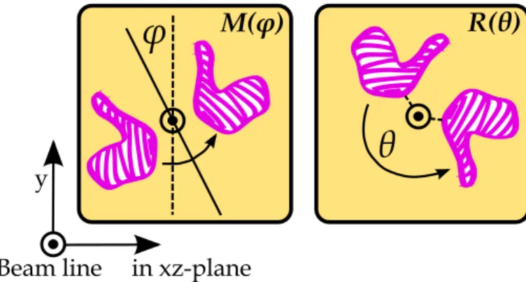
M(φ)and R(θ) in a plane orthogonal to a beam line. The beam line is pointing out of the paper. M(φ)is a reflection in a line making an angleφwith theyaxis. R(θ)is a rotation of an angleθ around the beam line.
First, we assume the pump field to be rotationally-symmetric with zero orbital angular momentum. Second, we consider only orthogonal image transformations which comprise any combination of image reflections and image rotations (see Fig. 2.2). We define M(φ) as an image reflection in a line oriented at an angle φwith respect to the y axis, and R(θ) as an image rotation over an angleθ. Finally, we assume one aperture to be fully open, i.e., T1(x1) = 1.
The first two restrictions allow us to combine all image operations into a single matrix Utot = U MyU My and reduce the two-photon amplitudes in Eq. (2.4) to
Ag(x1,x2) andAg(x1, Utotx2). The third restriction allows us to isolate the
trans-verse correlation function of the pump field. The expression for the two-photon bunching visibility thus becomes
V(θ) =
Z
˜ gz1
2(Utot−1)x2
T2(x2)dx2 Z
˜
gz(0)T2(x2)dx2
, (2.7)
where the normalized correlation function of the pump field (in spherical coordi-nates) is defined as
˜ gz(δx) =
Z
˜ E∗
z x+12δx ˜
Ez x−1 2δx
dx
Z
Ez˜ (x)
2
dx
. (2.8)
field ˜Ez(x) in spherical coordinates is related to the pump field in Cartesian coor-dinates as
˜
Ez(x)≡Ez(x) exp
−ikp2z|x|2
. (2.9)
Note that we have incorporated all phase factors in ˜Ez(x), by choosing a con-venient spherical coordinate system that has its origin at the center of the pump spot on the crystal. The pump profile ˜Ez(x) becomes real-valued in the far field, but is complex in the near field. As a result, only the far-field correlation function is directly related to the intensity profile of the pump in the detection plane. The near-field correlation function on the other hand is much narrower than the pump profile in the corresponding plane. For the experimentally important case of a Gaus-sian TEM00pump that is mildly focussed at the crystal asE0(x)∝exp (−|x|2/w02),
this correlation function is
˜
gz(x)∝exp
−|x|
2
2w2
z
1 + z
2 0
z2
, (2.10)
wherewz=w0 p
1 + (z/z0)2is width of the pump beam in the detection plane and
z0≡ 12kpw20 is the Rayleigh range of the pump beam.
There are two distinct possibilities for the orthogonal matrixUtot. If the built-in
operation in Fig 2.1 is an image rotationU = R(θ), the combined matrix Utot is
equal to unity and hardly interesting. If the built-in operation is an image reflection U = M(φ) =R(2φ)My, the combined operation Utot = R(4φ) is a rotation over
an angle 4φ. If the interferometer contains more than two mirrors, it can still be reduced to one of these two generic cases by absorbing the extra reflections in the effective image transformationU in Fig 2.1.
We will study the case where the effective image transformationU is an image reflection in more detail. We call this system an “odd-R” interferometer, to indicate that it operates as an interferometer containing an odd number of mirrors in between crystal and beam splitter and an image rotatorR(θ) = M(θ/2)My in one of its arms. We will evaluate Eq. (2.7) for this odd-R geometry, where the relationUtot=
R(2θ) yields
12(Utot−1)x2
= sinθ|x2|. We consider a geometry that comprises a
Gaussian TEM00 pump beam and a “hard-edged” circular aperture with a top-hat
transmission profileT2(x2) = Θ(1− |x2|/a) of radius apositioned in the far field of this beam (L0 ≫ z0). For this geometry, the two-photon bunching visibility
[Eq. (2.7)] becomes
V(θ) =1−exp (−ξ)
ξ , (2.11)
where ξ = 1 2(a/wz)
2sin2θ. Note that the predicted two-photon visibility V(θ) is
Our key result of Eq. (2.11) quantifies the effect of spatial labeling on the two-photon interference. If the aperture T2(x) is much smaller than the transverse
correlation length wz of the pump, we expect V(θ) ≈ 1 irrespective of the rota-tional angle θ, as the diffraction limit of the aperture frustrates the observation of any image rotation or reflection. If the aperture is much larger, diffraction will be less restrictive and V(θ) will decay rapidly away from θ = 0. The two-photon interference should disappear if one can distinguish the signal from the idler path based on any conceivable photon position measurement at the detector side, even if that measurement is not actually performed but only possible in principle. Mathe-matically, the criterion for spatial labeling translates into√2ξ= (a/wz) sin(θ)≫1.
2.3 Discrete modal analysis
2.3.1 Schmidt decomposition of the detected two-photon amplitude
In the previous section we have analyzed two-photon interference in a two-photon interferometer with an image transformation U in one of its arms (see Fig. 2.1). We considered the case of a rotationally symmetric pump profile and an orthogonal image transformation matrix U, comprising any combination of image reflections and rotations as visualized in Fig. 2.2. We found out that the two-photon bunching visibility is only affected byUifUis an image reflectionM(θ/2), which is equivalent to an image rotation in combination with an extra mirror R(θ)My. An expression forV(θ) is given by Eq. (2.11) for detection through a hard-edged circular aperture in front of one of the detectors. Our analysis that lead to this result was based on calculations of the continuous two-photon amplitude in the quasi-monochromatic paraxial thin-crystal limit.
In this subsection we will analyze the two-photon interference that leads to Eq. (2.11) from a different perspective, namely by decomposing the continuous two-photon amplitude into a countable set of discrete spatial modes. We will con-sider thedetected two photon amplitude [80] in stead of the generated two-photon amplitude [9, 81]. As we will show, the rotational symmetry of the pump and the apertures allows for a decomposition of the detected two-photon amplitude in a Fourier series of orbital angular momenta. This azimuthal decomposition is a first step towards a full Schmidt decomposition [9, 82, 83] of the detected field. Our Schmidt decomposition of the detected field is mathematically equivalent to the Schmidt decomposition of thegenerated field as performed in ref. [9].
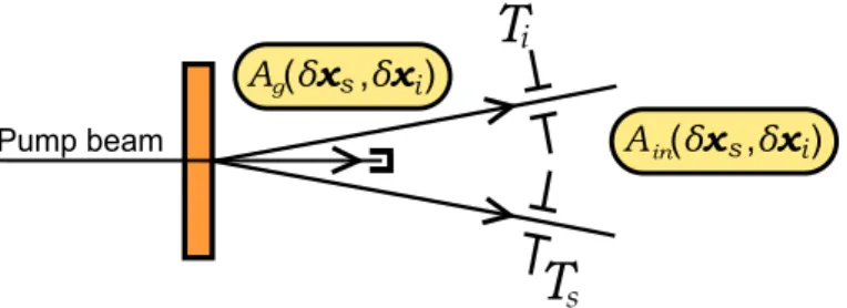
Figure 2.3: Graphical representation of what we call the detected two-photon amplitude
Ain(δxs, δxi)in relation to the generated two-photon amplitudeAg(δxs, δxi).
where φis the angle with the y axis and the sign of φ is defined in analogy with the definition ofR(θ) in Fig. 2.2. The detected two-photon amplitude is obtained by including the spatial filtering of two rotationally symmetric aperturesTs,i(rs,i) in the signal and idler beam (see Fig. 2.3). We analyze the angular dependence of this detected field by decomposing it in a Fourier series of orbital angular momenta l, via
Ain(rs, ri, φsi) ≡ p
Ts(rs)Ti(ri)Ag(rs, ri, φsi)
= A
∞
X
l=−∞
Fl(rs, ri)pPleilφsi/2π, (2.12)
whereA2≡RR
|Ain(δxs, δxi)|2dδxsdδxiis the average squared amplitude.
Further-more we haveFl(rs, ri) =F−l(rs, ri) and P−l =Pl, because of mirror symmetry. The functionsFl(rs, ri) are normalized via [9]
Z ∞
0
Z ∞
0 |
Fl(rs, ri)|2rsridrsdri= 1, (2.13)
so thatP
Pl= 1.
Equation (2.12) is a first step towards a full Schmidt decomposition of the de-tected two-photon amplitude. This decomposition can be completed by expand-ing [9]
Fl(rs, ri)√rsri=
∞
X
p=0
√γl,pfl,p(rs)gl,p(ri), (2.14)
where the radial mode numberpquantifies the number of nodal lines in the radial profile offl,p(rs) andgl,p(ri). The functionsfl,p(rs) andgl,p(ri) are normalized via the standard inner product so thatP
the detected two-photon amplitude now reads
Ain(δxs, δxi) =A
∞
X
l=−∞ ∞
X
p=0 p
λl,pul,p(δxs)v−l,p(δxi), (2.15)
where λl,p ≡ Plγl,p and ul,p(δxs) ≡ eilφsfl,p(rs)/ √
2πrs and vl,p(δxi) ≡ eilφigl,p(ri)/√2πri.
We now return to the HOM interference setup visualized in Fig. 2.1 with an image transformationU =R(θ)My. We reposition the aperturesTs(rs) andTi(ri) in front of the detectors 2 and 1, respectively. Because the generated fieldAg(δxs, δxi) is invariant under a coordinate swap δxs ↔ δxi, we can write the two-photon amplitude behind the apertures T1 and T2 in terms of the detected two-photon
amplitude, i.e.,
AHOM(x1,x2) = Tbse−i
1 2∆ωτA
in(r2, r1, φ1+φ2−θ)
−Rbsei
1 2∆ωτA
in(r2, r1, φ1+φ2+θ), (2.16)
where ∆ω ≡ ω1−ω2 is the angular frequency difference between photons 1 and
2 and τ ≡ (Ls−Li)/c is the time delay difference in the interferometer. The only difference between Eq. (2.4) and Eq. (2.16) is that the latter incorporates the transmission profiles of the detection apertures whereas Eq. (2.4) does not.
The two-photon bunching visibility as defined in Section 2.2 is now easily cal-culated by using the azimuthal Schmidt decomposition of the detected two-photon amplitude as given in Eq. (2.12). By substituting Eq. (2.12) in Eq. (2.16), assuming a balanced beam splitter Rbs =Tbs = 12, and using the prescriptions of Eqs. (2.5)
and (2.6) one quickly finds
V(θ) =
∞
X
l=−∞
Plcos (2lθ). (2.17)
In other words, a measurement ofV(θ) with the HOM setup as visualized in Fig. 2.1 (with U =R(θ)My) reveals the azimuthal Schmidt coefficients Pl of the detected two-photon amplitude. This key result will be discussed in more detail in Subsec-tion 2.3.3.
The OAM weightsPl depend on the size and radial shape of the circular de-tection apertures T1,2 in relation to the profile of the pump laser in the detection
plane, as these determine the detected two-photon amplitudeAin(rs, ri, φsi) and its
2.3.2 Modal decomposition and the Schmidt number
In this subsection we will introduce a convenient coordinate free bra-ket notation for the detected two-photon state (see Fig. 2.3) and use the Schmidt decomposition to quickly rederive the previous results of Eq. (2.16) and Eq. (2.17). We will also introduce two different Schmidt numbers.
A Schmidt decomposition of the detected two photon state|Ψiinin bra-ket form
is
|Ψiin= X
µ
p
λµ |uµi ⊗ |vµi, (2.18)
where {|uµi} and {|vµi} are two sets of orthogonal mode functions, which are identical only if the aperture profilesTsandTi are identical. The effective number of modes involved in this decomposition is defined by the so-called (2D) Schmidt number
K2D≡
P
µλµ
2
P
µλ2µ
. (2.19)
The rotation symmetry of the detected two-photon amplitude Ain(U δxs, U δxi) = Ain(δxs, δxi) allows one to separate the mode index µ
into an azimuthal mode numberland a radial mode numberp. It also enforces the conservation of OAM in the paraxial SPDC process [84] and changes the modal decomposition of Eq. (2.18) to
|Ψiin=
∞
X
l=−∞ ∞
X
p=0 p
λl,p|l, pi′⊗ | −l, pi′′, (2.20)
where|l, pi′ and| −l, pi′′are the LG-like Schmidt eigenmodes of the detected
two-photon amplitude. This equation is the bra-ket notation of Eq. (2.15), where|l, pi′
and| −l, pi′′correspond to the functionsul,p(δxs) andv
−l,p(δxi), respectively. As the amplitude coefficients p
λl,p already contain the effects of aperture filtering, they will decrease rapidly both for highpand highl values (highlstates are quite extended even forp= 0). We define the OAM probability asPl≡P
pλl,p and the related azimuthal Schmidt number as
Kaz ≡
1
P
lPl2
, (2.21)
for P
lPl = 1 ∗. The relation between the azimuthal Schmidt number Kaz and
the full 2D Schmidt numberK2D, depends on the radial profile of the detection
∗ The OAM probabilityP
land azimuthal Schmidt numberKaz that we introduce are closely
aperture.
We now return to the HOM interference setup visualized in Fig. 2.1 with an image transformation U. Starting from the modal decomposition of Eq. (2.20), it is relatively easy to apply the rotation and mirror operations that are needed to evaluate the doubly reflected and doubly transmitted field and the visibility of their interference. For the even-R geometry [U =R(θ)], the generated (l,−l) pairs are also detected as (l,−l) pairs behind the beam splitter and we expect good two-photon interference, i.e.,V(θ= 1), at any rotation angle. For the odd-R geometry [U = R(θ)My], the OAM inversion produced by the extra mirror leads to the detection of (l, l) and (−l,−l) pairs instead. As the OAM at the rotator is now different for the doubly reflected and doubly transmitted path, so is the effect of rotation. For rotation over an angleθ the combined two-photon state after HOM interference can now be written as
|ΨiHOM = X
l,p
h
Tbs p
λl,pe−i(lθ+1 2∆ωτ)
−Rbspλ−l,pei(lθ+
1 2∆ωτ)
i
|l, pi′⊗ |l, pi′′. (2.22)
This is the bra-ket notation of Eq. (2.16). Next, we assume a balanced beam splitter (Rbs =Tbs = 12) and use the reflection symmetry λl,p=λ−l,p (andPl =P−l) to obtain
V(θ) =
∞
X
l=−∞
Plcos (2lθ), (2.23)
where we normalized toP
lPl = 1 [equivalent toV(0) = 1]. With the convenient bra-ket notation, we thus recover the important Eq. (2.17) in only a few steps.
2.3.3 The physical significance of V(θ)
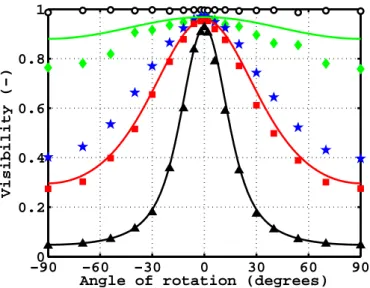
Equation (2.23) shows how the observed visibility V(θ) is a weighted sum over contributions from groups ofl modes, each contribution oscillating betweenVl= 1 (HOM dip) andVl=−1 (HOM peak) with its own angular dependence cos (2lθ). It thereby shows how the visibility V(θ) and the modal distribution{Pl} are related via a simple Fourier series. As a Fourier transformation ofV(θ) directly yields the full OAM distribution{Pl}, it thus provides for a complete characterization of the angular structure of the two-photon amplitude.
The azimuthal Schmidt numberKaz is a measure for the angular structure in
the detected two-photon amplitude. More precisely, by averaging V(θ)2 over the
full rotation range one finds
Kaz= P1
P2
l
= 1
WhenV(θ) remains close toV(0) = 1 over its full range, this relation givesKaz≈1.
WhenV(θ) = cos (2lθ) this relation gives Kaz = 2 as expected forPl=P−l = 12. WhenV(θ) ≈1 only in a very limited range aroundθ = 0 and zero for all other angles,Kaz≫1 is inversely proportional to the angular width ofV(θ).
In one of our experiments we use a single-mode detector that only selects photons with a specific OAM valueld. We predict that the coincidence rate versus time delay Rcc(θ, τ) now contains both a symmetric and (surprisingly) also an anti-symmetric
part with respect to time delayτ. Using the detected two-photon state after HOM interference of Eq. (2.22) for a singlel=ld number we find
Rcc(θ, τ)∝ Z
[1 + cos(∆ωτ + 2ldθ)]Ttot(∆ω)d∆ω, (2.25)
whereTtot(∆ω) is defined below Eq. (2.5). This equation shows thatRcc(θ, τ) will
have an antisymmetric component with respect toτonly ifTtot(∆ω) is asymmetric
and if sin(2lθ)6= 0. Note thatTtot(∆ω) is only asymmetric if the filter transmission
spectraTf1(ω) andTf2(ω) are different. For the two-photon bunching visibility at
zero delay, which solely depends on the symmetric part, we find the earlier result of Eq. (2.23), which now reduces toV(θ) = cos (2ldθ).
Finally, one might wonder what the observed visibilityV(θ) tells us about the nature of the spatial entanglement, i.e., whether it proofs that the two-photon am-plitude is indeed described by the pure state of Eq. (2.20) with its perfect OAM entanglement? This question is best answered by arguing backwards from hypo-thetical detected pairs (l1, l2). For an even-R interferometer, our experimental
ob-servation thatV(θ)≈1 irrespective of rotation angle indeed proofs the conservation of OAM; it shows that the two-photon field at the detectors contains only (l,−l) pairs, as any other pairs (l1, l2) would introduce an angle dependence of the form
cos (2(l1+l2)θ) in V(θ). However, as the same result V(θ) ≈1 would have been
obtained for any classical mixture of (l,−l) pairs, this observation doesn’t proof the existence of quantum entanglement. For the odd-R interferometer, the observations onV(θ) discussed in this chapter does proof some form of quantum entanglement. It shows that the two-photon amplitude contains only coherent superpositions of the form|Ψi=|l,−li+| −l, li. Again, we cannot exclude any incoherent mixture of these superposition states.
2.4 Experimental results
2.4.1 Experimental setup
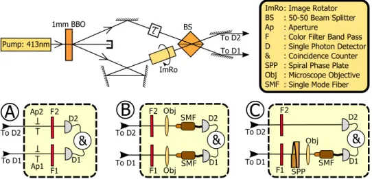
Figure 2.4: Experimental setup: A two-photon interferometer with an odd number of mirrors and a built-in image rotator. Theτ-icon represents an adjustable delay line. Behind the beam splitter three different detection geometries can be chosen: A, B, or C.
in a vertically polarized pure TEM00 mode. The beam is mildly focussed (wp =
270µm is the radius at e−2 of maximum irradiance) on a 1 mm thickβ-BaB 2O4
crystal (BBO) with a cutting angle of 29.2◦. The crystal is tilted such that we obtain
type I spontaneous parametric down conversion (SPDC) where the SPDC light is emitted in a cone extending over a full opening angle of 2θ0= 3.2◦around the pump
beam. After multiple reflections and a single transit through the image rotator, two opposite parts of this cone are combined on a beam splitter. The crucial angular alignment of this beam splitter is performed with computer-controlled actuators. Behind the 50/50 beam splitter, three different detection geometries can be chosen (described in more detail in the next paragraph). Color filters are positioned in front of the detectors in all detection geometries. The filters are custom-made bandpass filters (Chroma Technology Corporation), filtering around 826 nm with a FWHM of 5 nm. The detectors in all three detection geometries are single photon sensitive avalanche photodiodes (Perkin Elmer SPCM-AQR-14).
Figure 2.5: Scheme of the different components of our image rotator, drawn in thexzplane (see Fig 2.1). Light enters with an in-plane linear polarization. The rotatable part (drawn here in theφ = 0 situation) can be rotated as a whole around the indicated axis, and it is responsible for an image reflection M(φ) as defined in Fig. 2.2. The polarizer selects the in-plane polarization.
fabrication of the SPP can be found in Subsection 2.4.2. The apertures (in geometry A) and the position of the objectives (in geometries B and C) define the signal and idler path. The beam splitter is positioned on the crossing of the signal and idler path and is angle tuned such that the detection apertures obey mirror symmetry with respect to the beam splitter plane. The signal and idler arm of the interfer-ometer each have a length of 1.6 m. The direction of the pump beam is centered in between the directions of the signal and idler path. The idler arm contains a delay line with which the length of the arm, and hence the relative arrival times of the photons at the beam splitter, can be adjusted.
The microscope objectives in detection geometry B are Leica 10x/0.25 infinity-corrected objectives with an effective focal length of 20 mm. They are positioned at 0.6 m from the beam splitter and image the tip of the single-mode fiber (Thorlabs SM800-5.6-125) onto the BBO crystal. The radius (at e−2 of maximum
irradi-ance) of this image of the detected mode on the BBO crystal is measured to be 280µm. We use slightly different optics in detection geometry C, in order to ob-tain a narrower waist of the detected mode on the BBO crystal. The radius (at e−2 of maximum irradiance) of the detectedl = 0 mode, i.e. whenever the SPP is
temporally removed from the apparatus, on the BBO crystal is now 220µm. The radius of the characteristic ring of the detectedl= 1 mode, i.e. whenever the SPP is in the apparatus, is 180µm. This value is somewhat larger than the value of
1 2
√
2×220µm = 156µm expected for the (l= 1,p= 0) mode due to the presence of higher orderpmodes.
the far field and±0.5 mm in the near field, measured over a full rotation. The fixed mirror on the left causes an image reflectionM(0) so that the combined action of the unit is a rotationR(θ) =R(2φ) =M(φ)M(0).
Although an image rotation is generally accompanied by a polarization rota-tion [86], our rotator transfers at most only 8% of the power into the orthogonal polarization. This convenient property is obtained by using silver mirrors (protected by a thin SiO2 cover layer) instead of dielectric mirrors. The measured phase
dif-ference between the (three-fold) reflected s- and p-polarized light is φs−p = 0.81π, which is sufficiently close to the ideal value of φs−p=π needed for a polarization-insensitive rotator∗. As both polarization components have the same spatial profile,
we simply remove this small unwanted orthogonal component with a fixed polarizer (see Fig. 2.5).
2.4.2 Spiral phase plate
A spiral phase plate (SPP) is a transparent plate whose thickness increases pro-portional to the azimuthal angle [87]. It imposes an azimuth-dependent optical retardation on the optical field. Our SPP is custom made by Philips Research Laboratories with dimensions suited for our application; the imposed optical retar-dation over a full rotation equals one optical cycle of the 826.2 nm SPDC light. The SPP operates as a lowering operator on l-numbers of the incoming modes at this wavelength. In detection geometry C, a single-mode fiber is used to detect solely the fundamental Gaussian mode (l= 0) behind the SPP which implies that it solely detects an l= 1 mode in front of the SPP.
The SPP is manufactured using photo replication technology [88]. To this end a high accuracy brass mould, the negative of the SPP we wish to produce, is machined using a programmable computer driven diamond tool. A transparent copy of the mould is obtained by using a reactive monomer encapsulated between the mould and a cover glass plate. The final SPP is obtained after polymeriza-tion of the monomer by UV radiapolymeriza-tion. The demand for an optical retardapolymeriza-tion of 826 nm in one cycle requires proper definition of step height and refractive index. We use a step height of 1.66 µm and a refractive index of 1.50. Some technical details on the production process are as follows: We use an adhesion promoter γ-(methacryloyloxypropyl)trimethoxysilane to allow for a firm coupling between the resulting polymer and the cover. We use a mixture of poly(ethyleneglycol) dimethacrylate with a refractive index of 1.48 and Ebecryl 604 (75% epoxyacrylate in hexanedioldiacrylate, a product of UCB chemicals) with a refractive index of 1.54 in a ratio of 2 : 1 to obtain an effective index of 1.50. To enable the