AIP Conference Proceedings 2070, 020044 (2019); https://doi.org/10.1063/1.5090011 2070, 020044 © 2019 Author(s).
Towards single- and multiobjective Bayesian
global optimization for mixed integer
problems
Cite as: AIP Conference Proceedings 2070, 020044 (2019); https://doi.org/10.1063/1.5090011
Published Online: 12 February 2019
Kaifeng Yang, Koen van der Blom, Thomas Bäck, and Michael Emmerich
ARTICLES YOU MAY BE INTERESTED IN
The R2 indicator: A study of its expected improvement in case of two objectives
AIP Conference Proceedings 2070, 020054 (2019); https://doi.org/10.1063/1.5090021
Towards self-adaptive efficient global optimization
AIP Conference Proceedings 2070, 020056 (2019); https://doi.org/10.1063/1.5090023
On the hierarchical structure of Pareto critical sets
Towards Single- and Multiobjective Bayesian Global
Optimization for Mixed Integer Problems
Kaifeng Yang
a), Koen van der Blom
b), Thomas B¨ack
c)and Michael Emmerich
d)LIACS, Leiden University, Niels Bohrweg 1, 2333CA Leiden, Netherlands
a)Corresponding author: [email protected] b)[email protected]
c)[email protected] d)[email protected]
Abstract.Bayesian Global Optimization (BGO) is a very efficient technique to optimize expensive evaluation problems. However, the application domain is limited to continuous search spaces when using a BGO algorithm. To solve mixed integer problems with a BGO algorithm, this paper adapts the heterogeneous distance function to construct the Kriging models and applies these new Kriging models in Multi-objective Bayesian Global Optimization (MOBGO). The proposed mixed integer MOBGO algorithm and the traditional MOBGO algorithm are compared on three mixed integer multi-objective optimization problems (MOP), w.r.t. the mean value of thehypervolume(HV) and the related standard deviation.
ALGORITHM
Bayesian Global Optimizationwas proposed by the Lithuanian research group of Jonas Mockus and Antanas ˇZilinskas [1, 2]. The basic idea of BGO, also known asEfficient Global Optimization, is to build a statistical model to reflect the relationship between decision vectorsX = (x(1),x(2),· · ·,x(n))> in anm dimensional search space, and their
corresponding objective valuesY(X)=(y(x(1)),y(x(2)),· · ·,y(x(n)))>. Then an optimizer in a BGO algorithm searches
for an optimal solution by using the predictions of the surrogate model(s), instead of evaluating the real objective function.
To construct a surrogate model, it is assumed that the objective function is the realization of a Gaussian random field, which is also called Gaussian processes (GP) or Kriging in BGO. Specifically, Kriging assumes yto be a realization of a random processY and to be of the form [3]:
Y(x)=µ(x)+(x) (1)
whereµ(x) is the estimated mean value over all given sampled points, and(x) is a realization of a normally distributed Gaussian random process with a zero mean and a variance ofσ2. The correlation between the deviations at two points (xandx0) using an isotropic Gaussian Kernel is defined as:
Corr[(x), (x0)]=R(x,x0)=exp−θd(x,x0)2 (θ>=0) (2) whereR(·,·) is the correlation function, andd(·,·) is the Euclidean distance function.
In Kriging, the distance value between two points is usually calculated with the Euclidean metric, that isd(x,x0)=
q Pi=m
i=1(xi−x
0
i)
2. This is useful and straightforward in a continuous search space, as the Euclidean metric assumes the continuity of an objective function. However, this assumption will not be suitable when the search space is a nominal discrete or an integer space.
To solve this problem, we applied the heterogeneous metric [4, 5] as the distance function, which is defined as:
dh(x,x0)=
v u ti=nr
X
i=1 (ri−r
0
i)2+ i=nz X
i=1 |zi−z
0
i|+ i=nd X
i=1
I(di,d 0
whereI(true)=1 andI(f alse)=0. The idea of the heterogeneous metric is to combine different metrics by taking the square root of the sum of each distance. As shown in Eq. (3), the distance between any two points in a nominal discrete space and an integer space is measured by the overlap metric and the Manhattan metric, respectively. A detailed motivation of the heterogeneous metric in the context of statistical modeling is provided in [5].
TEST PROBLEMS
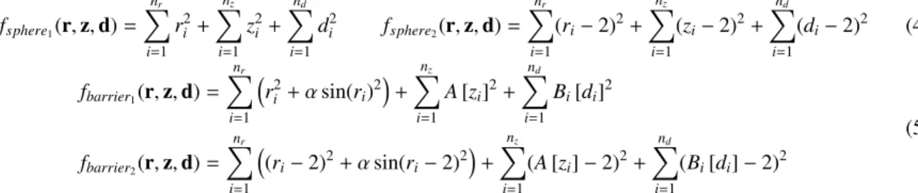
Three mixed integer MOPs are used in this paper, specifically: the double sphere function in Eq. (4) [5], the double barrier function in Eq. (5) [6], and a multi-layer optical filter optimization problem [7].
fsphere1(r,z,d)= nr X
i=1
ri2+
nz X
i=1
z2i +
nd X
i=1
d2i fsphere2(r,z,d)= nr X
i=1
(ri−2)2+ nz X
i=1
(zi−2)2+ nd X
i=1
(di−2)2 (4)
fbarrier1(r,z,d)= nr X
i=1
r2i +αsin(ri)2
+
nz X
i=1
A[zi]2+ nd X
i=1
Bi[di]2
fbarrier2(r,z,d)= nr X
i=1
(ri−2)2+αsin(ri−2)2
+
nz X
i=1
(A[zi]−2)2+ nd X
i=1
(Bi[di]−2)2
(5)
In Eq. (4) and Eq. (5),r,z, anddrepresent a real variable vector, an integer variable vector, and a nominal discrete variable vector, respectively.
For the barrier functionα =1, andAis generated by Algorithm 6 from Li et al (2013) [6] with the parameter
C=75, andBi∈1,...,ndis a set ofndrandom permutations of the sequence 0, . . . ,4. BothAandBremain fixed throughout
the experiments. Unlike in [6], here smooth wave-like barriers are used in the real part, rather than staircase-like barriers. For the multi-objective case both of these functions can be adjusted with an offset for each term, such that real, integer, and nominal discrete optima are different in the second objective.
For the optical filter problem [7], the pairs of continuous and (binary) nominal discrete variables are considered. When the binary variable is active the corresponding continuous variable is used in the objective functions, otherwise it is ignored. If all bits are inactive a penalty of (250,1250) is returned. In addition to the original objective we consider
fopt f ilt2(r,d)=
Pnr
i=1ridias a second objective. The parameters of each test problem are given in Table 1.
RESULTS
All the experiments are performed on the same computer: Intel(R) i7-4800mq CPU @ 2.70GHz, RAM 32GB. The operating system is Ubuntu 16.04 LTS (64 bit), and the platform is MATLAB 8.4.0.150421 (R2014b), 64 bit.
Figure 1 shows the heatmap comparison of the predictions by using different distance metrics for the barrier function in Eq. (5). For the visualization, only one variable is considered for each variable type. The parameterθin Eq. (2) is chosen asθ=[0.01,0.01,0.01]. Each variable is normalized to [0,1] in Figure 1. The number of sampling points is 15 and there are 200 random points for the test points. Note that the pictures in the third column don’t have sampling points and are plotted with these 200 test points, which are evaluated on the real objective functions. These 200 test points are used to visualize the landscape of the barrier function. In these figures, the models using the heterogeneous metric are more accurate than those using the Euclidean metric, especially in the fbarrier1function.
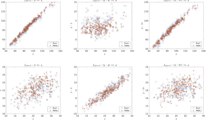
Figure 2 illustrates the comparison of the predictions of the sphere functions using the Euclidean metric and the heterogeneous metric. There are 15 variables in total, 5 variables for each type. The number of sampling points is 90 and the number of test points is 200. The optimalθin the Kriging models are calculated with the simplex search method of Lagarias et al. (f minsearch) [8], with the parameter of max function evaluations as 1000. In Figure 2, ˆy
andσrepresent the predicted mean and the predicted standard deviation, respectively. After applying the optimalθ strategy for both the Euclidean metric and the heterogeneous metric, the prediction of using the Euclidean metric is similar to that of using the heterogeneous metric. However, the Kriging models using the heterogeneous metric still outperform the Kriging models using the Euclidean metric, w.r.t. the standard deviation of the predictions.
FIGURE 1.Landscape of the fmbarrierfunction
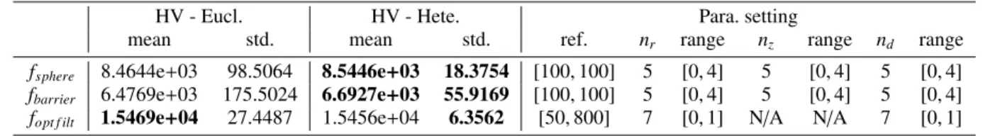
both algorithms, the optimalθcalculated by f minsearch[8] are used, the infill criterion is theExpected Hypervolume Improvement [9] and the optimizer is a build-in genetic algorithm [10] in MATLAB. The results in Table 1 show that the mixed integer MOBGO using the heterogeneous metric outperforms the traditional MOGBO on both the barrier and sphere test problems, w.r.t. mean hypervolume (HV) values and the standard deviations of the HV over 10 repetitions. For the optical filter problem, the traditional MOBGO can generate a better Pareto front set, but the mixed integer MOBGO is more robust than the traditional MOBGO, w.r.t. standard deviation.
TABLE 1.Parameter settings and empirical experimental results
HV - Eucl. HV - Hete. Para. setting
mean std. mean std. ref. nr range nz range nd range
fsphere 8.4644e+03 98.5064 8.5446e+03 18.3754 [100,100] 5 [0,4] 5 [0,4] 5 [0,4]
fbarrier 6.4769e+03 175.5024 6.6927e+03 55.9169 [100,100] 5 [0,4] 5 [0,4] 5 [0,4]
fopt f ilt 1.5469e+04 27.4487 1.5456e+04 6.3562 [50,800] 7 [0,1] N/A N/A 7 [0,1]
CONCLUSIONS AND FUTURE WORK
This paper proposes a mixed integer MOBGO by using the heterogeneous metric, instead of the Euclidean metric. Both of these two algorithms are compared in terms of the prediction errors and performance of the final Pareto front sets on three mixed integer multi-objective test problems. The results show that the proposed method surpasses the traditional MOBGO on both sphere and barrier test functions, with regard to the prediction errors, mean HV and standard deviation of the HV. On the optical filter problem, the traditional MOBGO performs slightly better than the proposed algorithm. The reason for this could be thatNmaxis too small, as this problem contains 14 variables.
FIGURE 2.Comparison of predictions on fmspherefunctions
REFERENCES
[1] A. ˇZilinskas and J. Mockus, Avtomatica i Vychislitel’naya Teknika4, 42–44 (1972).
[2] J. Moˇckus, “On bayesian methods for seeking the extremum,” inOptimization Techniques IFIP Technical Conference Novosibirsk, July 1–7, 1974, edited by G. I. Marchuk (Springer Berlin Heidelberg, Berlin, Hei-delberg, 1975), pp. 400–404.
[3] D. R. Jones, M. Schonlau, and W. J. Welch,Journal of Global optimization13, 455–492 (1998). [4] D. R. Wilson and T. R. Martinez,Journal of artificial intelligence research6, 1–34 (1997).
[5] R. Li, M. T. M. Emmerich, J. Eggermont, E. G. P. Bovenkamp, T. Back, J. Dijkstra, and J. H. C. Reiber, “Metamodel-assisted mixed integer evolution strategies and their application to intravascular ultrasound im-age analysis,” in2008 IEEE Congress on Evolutionary Computation (IEEE World Congress on Computa-tional Intelligence)(2008), pp. 2764–2771.
[6] R. Li, M. T. M. Emmerich, J. Eggermont, T. B¨ack, M. Sch¨utz, J. Dijkstra, and J. H. C. Reiber,Evolutionary computation21, 29–64 (2013).
[7] J.-M. Yang and C.-Y. Kao, “An evolutionary algorithm for synthesizing optical thin-film designs,” inParallel Problem Solving from Nature — PPSN V, edited by A. E. Eiben, T. B¨ack, M. Schoenauer, and H.-P. Schwefel (Springer Berlin Heidelberg, Berlin, Heidelberg, 1998), pp. 947–956.
[8] J. C. Lagarias, J. A. Reeds, M. H. Wright, and P. E. Wright,SIAM Journal on Optimization9, 112–147 (1998), https://doi.org/10.1137/S1052623496303470 .
[9] M. Emmerich, K. Yang, A. Deutz, H. Wang, and C. M. Fonseca, inAdvances in Stochastic and Deterministic Global Optimization, edited by P. M. Pardalos, A. Zhigljavsky, and J. ˇZilinskas (Springer, Berlin, Heidelberg, 2016), pp. 229–243.
[10] D. E. Goldberg,Genetic Algorithms in Search, Optimization and Machine Learning, 1st ed. (Addison-Wesley Longman Publishing Co., Inc., Boston, MA, USA, 1989).