Printed in Great Britain Advance Access publication 10 August 2016
Variable selection for case-cohort studies with failure
time outcome
BYAI NI, JIANWEN CAIANDDONGLIN ZENG
3101 McGavran-Greenberg Hall, CB 7420, Department of Biostatistics, University of North Carolina at Chapel Hill, Chapel Hill, North Carolina 27599, U.S.A.
[email protected] [email protected] [email protected]
SUMMARY
Case-cohort designs are widely used in large cohort studies to reduce the cost associated with covariate measurement. In many such studies the number of covariates is very large, so an effi-cient variable selection method is necessary. In this paper, we study the properties of a variable selection procedure using the smoothly clipped absolute deviation penalty in a case-cohort design with a diverging number of parameters. We establish the consistency and asymptotic normality of the maximum penalized pseudo-partial-likelihood estimator, and show that the proposed vari-able selection method is consistent and has an asymptotic oracle property. Simulation studies compare the finite-sample performance of the procedure with tuning parameter selection meth-ods based on the Akaike information criterion and the Bayesian information criterion. We make recommendations for use of the proposed procedures in case-cohort studies, and apply them to the Busselton Health Study.
Some key words: Case-cohort design; Diverging number of parameters; Oracle property; Smoothly clipped absolute deviation; Survival analysis; Variable selection.
1. INTRODUCTION
Large-scale epidemiological studies and disease prevention trials often follow thousands of subjects for long periods of time. Measuring covariates for the entire study cohort can be pro-hibitively expensive, especially when it involves taking biological samples or performing expen-sive bioassays. Moreover, the rate of occurrence of the event of interest, such as cardiovascular disease, stroke or death, is typically low in such studies. We refer to subjects who develop the event of interest during the study as cases and the other subjects as noncases. If the covariates were to be measured for everyone in the study, most of the cost would be spent on the noncases, who do not contribute as much information as the cases. To reduce the cost and effort in collect-ing expensive covariates while loscollect-ing as little efficiency as possible,Prentice(1986) proposed the case-cohort design, where complete covariate information is obtained from only a random subcohort of the sample, as well as from all of the cases.
Various estimation methods have been developed for case-cohort studies under the propor-tional hazards model (Cox,1972).Prentice(1986) andSelf & Prentice(1988) proposed a pseudo-partial-likelihood method that modifies the risk set to account for subcohort sampling.Barlow
(1994) introduced a time-dependent weight to estimate the risk set from the subcohort sample and developed a robust variance estimator for the regression parameters.Kalbfleisch & Lawless
(1988) proposed a more efficient weighting that uses the complete covariate history of all cases.
Borgan et al. (2000) further studied several types of weights under the stratified case-cohort
c
design. Kulich & Lin(2004) established the asymptotic properties of the efficiently weighted estimator ofKalbfleisch & Lawless(1988);Kang & Cai(2009) extended this estimator to stud-ies with multivariate failure time outcomes, andKim et al.(2013) further improved the estima-tor’s efficiency in the presence of multivariate failure time outcomes. In this paper, we focus on the efficient weighting proposed by Kalbfleisch & Lawless(1988) in a univariate unstratified case-cohort design.
In large epidemiological studies that use the case-cohort design, many covariates are usually collected, and often one goal of the research is to identify a subset of covariates related to the event of interest. With the inclusion of interactions and polynomial terms, the number of candi-date covariates can be very large. AsHuber(1973) argued, in the context of variable selection, the number of parameters should be considered as increasing to infinity with the sample sizen. In this paper, we consider the scenario where the model sizedndiverges to infinity but at a slower rate than the sample size. Traditional variable selection methods such as stepwise and best subset selection are computationally intensive and unstable. Since the introduction of the lasso by Tib-shirani(1996), penalty-based variable selection procedures have achieved great success. Under certain regularity conditions, these methods can simultaneously select variables and estimate their coefficients. Many penalty functions have been proposed, among which the smoothly clipped absolute deviation (Fan & Li, 2001), adaptive lasso (Zou, 2006), adaptive elastic net (Zou & Zhang,2009) and minimax concave (Zhang,2010) penalties have been shown to possess the ora-cle property, namely, asn→ ∞the procedure correctly identifies the true model with probability tending to unity and estimates the standard errors of nonzero parameters as efficiently as if the true model were known.Fan & Li(2002) applied the smoothly clipped absolute deviation penalty to the proportional hazards model and proved its oracle property.Cai et al.(2005) extended the penalized partial likelihood procedure to multivariate models with a diverging number of param-eters. However, to the best of our knowledge, the properties of penalized variable selection have not been studied under the case-cohort design where not all covariates are fully observed.
2. PSEUDO-PARTIAL LIKELIHOOD FOR CASE-COHORT DESIGNS
Suppose there arenindependent subjects in a cohort. LetZi(t)be thedn×1, possibly time-dependent, covariate vector for subjectiat timet. Sincedn goes to infinity withn, all quantities that are functions of the covariates depend on n. For notational simplicity, however, we shall suppress the subscriptn. Without loss of generality, we partition the real-valued true parameter vectorβn0as(βnT0,I, βnT0,II)T, whereβn0,Iandβn0,IIare the nonzero and zero components ofβn0,
respectively. Denote bykn the dimension ofβn0,I, which is allowed to diverge withnin such a
way thatkn/dnconverges to a constantc∈[0,1].
LetT andC be, respectively, the time to the outcome of interest and the censoring time. Let X=min(T,C)be the observed time and let=I(T C) be the censoring indicator, where I(·) denotes the indicator function. We assume thatT and C are independent, conditional on Z. Define for subjecti the counting process Ni(t)=I(Xit, i =1)and the at-risk process Yi(t)=I(Xi t). Letλi(t)denote the hazard function for subjecti.Cox(1972) proposed the proportional hazards modelλi{t|Zi(t)} =λ0(t)exp{βTZi(t)}, in whichλ0(t)is an unspecified
baseline hazard function.
If complete covariate histories are available for all the cases, one can use the following pseudo-partial likelihood to estimate the regression coefficientsβ(Kalbfleisch & Lawless,1988):
˜ n(β)=
n
i=1
τ
0
⎡ ⎣βT
Zi(t)−log n
j=1
ρj(t)Yj(t)exp{βTZj(t)} ⎤
⎦dNi(t), (1)
where τ is the time at the end of the study and ρi(t)=i +(1−i)ξiαˆ−1(t), with
ˆ
α(t)=ni=1(1−i)ξiYi(t)/{ n
i=1(1−i)Yi(t)} being a time-dependent estimator of the true sampling probabilityα. The corresponding pseudo-partial score equation is
˜ n(β)=
n
i=1
τ
0
Zi(t)−
˜
S(1)(β,t)
˜
S(0)(β,t)
dNi(t)=0,
where S˜(k)(β,t)=n−1ni=1ρi(t)Yi(t)Zi(t)⊗kexp{βTZi(t)} for k=0,1,2. Here a⊗0=1, a⊗1=aanda⊗2=aaTfor a vectora.
3. VARIABLE SELECTION WITH A PENALIZED PSEUDO-PARTIAL LIKELIHOOD 3·1. Penalized pseudo-partial likelihood
We define a penalized pseudo-partial likelihood as
˜
Qn(β)= ˜n(β)−n dn
j=1
Pλn j(|βj|), (2)
where Pλn j(|βj|) is a nonnegative penalty function with Pλn j(0)=0. The nonnegative tuning
parameterλn j controls the model complexity. We use the smoothly clipped absolute deviation penalty (Fan & Li,2001) with covariate-specific tuning parametersλn j, which allows different regression coefficients to have different penalty functions. The smoothly clipped absolute devi-ation penalty is
Pλn j(θ)= ⎧ ⎪ ⎪ ⎪ ⎪ ⎪ ⎪ ⎨ ⎪ ⎪ ⎪ ⎪ ⎪ ⎪ ⎩
λn jθ, θλn j,
−θ
2−2aλ
n jθ+λ2n j
2(a−1) , λn j < θaλn j, (a+1)λ2n j
2 , θ >aλn j, for somea>2 andθ >0. The first derivative of the penalty is
Pλn j(θ)=λn jI(θ λn j)+ (
aλn j−θ)+
a−1 I(θ > λn j). 3·2. Regularity conditions
For eachn, we define
Sn(k)(βn,t)= 1 n
n
i=1
Yi(t)Zi(t)⊗kexp{βnTZi(t)} (k=0,1,2),
en(βn,t)=sn(1)(βn,t)
sn(0)(βn,t),
Vn(βn,t)=
Sn(2)(βn,t)Sn(0)(βn,t)−Sn(1)(βn,t)⊗2 Sn(0)(βn,t)2
,
˜
Vn(βn,t)=
˜
Sn(2)(βn,t)S˜n(0)(βn,t)− ˜Sn(1)(βn,t)⊗2
˜
Sn(0)(βn,t)2
,
In(βn)=E
τ
0
Vn(βn,t)Sn(0)(βn,t)d0(t)
,
n(βn)=var
n−1/2˜n(βn)
.
We require the following regularity conditions:
Condition1. 0τ λ0(t)dt<∞andE{Y(τ)}>0;
Condition2. |Zi j(0)| + τ
0|dZi j(t)|<C1<∞ almost surely for some constant C1, for
i=1, . . . ,nand j=1, . . . ,dn;
Condition3. there exists a neighbourhood Bn of βn0 such that for all βn∈Bn and t∈ [0, τ], ∂sn(0)(βn,t)/∂βn=sn(1)(βn,t) and ∂2sn(0)(βn,t)/(∂βn∂βnT)=s(
2)
n (βn,t). The functions sn(k)(βn,t)(k=0,1,2) are continuous and bounded, andsn(0)(βn,t)is bounded away from zero onBn×[0, τ];
Condition4. there exist positive constantsC2,C3,C4andC5such that
0<C2< λmin{In(βn0)}λmax{In(βn0)}<C3<∞,
0<C4< λmin{n(βn0)}λmax{n(βn0)}<C5<∞,
whereλmin(·)andλmax(·)are the minimum and maximum eigenvalues of a matrix;
Condition5. min1jkn|βn j0|/λn j→ ∞asn→ ∞;
Condition6. lim infn→∞lim infθ→0+Pλn j(θ)/λn j>0 for j=1, . . . ,dn.
Condition1guarantees a finite baseline cumulative hazard and a nonempty risk set at the end of the study. Condition2requires the stochastic process of each time-dependent covariate to have bounded variation almost surely. Condition3essentially requires exp{βT
nZi(t)}to be integrable under a diverging dimension so that integration and differentiation with respect to Sn(k)(βn,t) (k=0,1) can be interchanged. Condition4 ensures that the covariance matrices of the score function under both regular and case-cohort designs are positive definite and have uniformly bounded eigenvalues for alln; it assumes a nonsingular Hessian matrix of the objective function used for variable selection. The same condition has been assumed in other works on variable selection (Peng & Fan,2004;Cai et al.,2005;Cho & Qu,2013). Condition5specifies the rate at which the proposed procedure can distinguish nonzero parameters from zero ones. Asn→ ∞, the size of nonzero parameters detectable by the procedure can approach zero, but at a slower rate than the tuning parameter. This condition is required for the derivation of the asymptotic properties of the proposed procedure, and has been assumed by many authors (e.g.,Peng & Fan,
there usually exists a fixed minimum clinically important effect size. Any effect smaller than this size can effectively be treated as zero. Thus, Condition5is a reasonable requirement. Condition6
implies that those zero parameters whose finite-sample estimates are of about the same scale as theλn jwill automatically be shrunk to zero; this helps to establish the oracle property of variable selection.
3·3. Asymptotic properties
Throughout this paper we use Op(·)andop(·)to denote probability order relations andO(·)
and o(·) to denote almost-sure order relations. Let an=max1jkn{|Pλn j(|βn j0|)|} and bn=
max1jkn{|Pλn j(|βn j0|)|}. We first prove the existence of a penalized pseudo-partial-likelihood
estimator that converges at rateOp{dn1/2(n−1/2+an)}and then establish its oracle property. The proofs of Theorems1and2are provided in the Appendix.
THEOREM1. Under Conditions1–5, if bn→0 and dn4/n→0as n→ ∞, then with proba-bility tending to 1there exists a local maximizerβˆn ofQ˜n(βn)= ˜n(βn)−n
dn
j=1Pλn j(|βn j|)
such that ˆβn−βn0 =Op{d 1/2
n (n−1/2+an)}.
From Theorem 1one can obtain a(n/dn)1/2-consistent penalized pseudo-partial-likelihood estimator, provided that an=O(n−1/2), which is the case for the smoothly clipped absolute deviation penalty under Condition5. This consistency rate is the same as that of the maximum likelihood estimator for the exponential family (Portnoy,1988). For the next theorem, we define
n=diag{Pλ1n(|βn01|), . . . ,Pλkn n(|βn0kn|)}, (3)
Bn= {Pλ1n(|βn01|)sgn(βn01), . . . ,Pλkn n(|βn0kn|)sgn(βn0kn)}
T. (4)
THEOREM2. Under Conditions1–6, if bn→0, dn5/n→0,λn j→0,λn j(n/dn)1/2→ ∞and an=O(n−1/2)as n→ ∞, the(n/dn)1/2-consistent local maximizerβˆn=(βˆnT,I,βˆnT,II)Tmust be such thatβˆn,II=0with probability tending to unity and, for any nonzero kn×1constant vector
un withun =1,
n1/2uT
n−
1/2
n11 (In11+n){ ˆβn,I−βn0,I+(In11+n)−1Bn} →N(0,1)
in distribution, wherenand Bnare defined in(3)and(4), respectively, In11consists of the first
kn×kn components of In(βn0), andn11consists of the first kn×kn components ofn(βn0).
Because of the diverging dimension ofβn0,I, Theorem2establishes the asymptotic normality
of some linear combination of standardized estimators. However, by choosing a particularun, it can give the asymptotic distribution of each individual estimator. Thus, it provides a theoretical basis for inference on individual coefficients. The matrixIn(βn0)can be consistently estimated
by Inˆ (βˆn)=n−1 n
i=1
τ
0 Vn˜ (βˆn,t)dNi(t). The estimator of the matrixn(βn0)is given in the
Supplementary Material. For the smoothly clipped absolute deviation penalty, an=0, n=0 and Bn=0 for largen under Condition5. Therefore, the result of Theorem2reduces to
n1/2uT
n−
1/2
n11 In11(βˆn,I−βn0,I)→N(0,1)
4. PRACTICAL IMPLEMENTATION CONSIDERATIONS 4·1. Local quadratic approximation and variance estimation
Since the smoothly clipped absolute deviation penalty function is not differentiable at the ori-gin, in practical implementations the Newton–Raphson algorithm cannot be applied directly to maximize (2). Instead, we use a modified Newton–Raphson algorithm with a local quadratic approximation to the penalty function. The unpenalized pseudo-partial likelihood (1) can be seen as a special case of the penalized pseudo-partial likelihood (2) with Pλn j(|βn j|)=0 for all j=1, . . . ,dn. Applying Theorem1withλn j=0 for all j=1, . . . ,dn, we know there exists a (n/dn)1/2-consistent maximizer of (1). The concavity of (1) ensures that the maximizer is unique. We use this maximizer as the initial value βn(0) for the modified Newton–Raphson algorithm. If |βn j(0)|is less than a prespecified small positive constant cj, then we set βˆn j =0. Otherwise, the penalty function is locally approximated by a quadratic function, Pλn j(|βn j|)≈ Pλn j{|βn j(0)|} + Pλn j{|βn j(0)|}{2|βn j(0)|}−1[βn j2 − {βn j(0)}2], which has the same value and first deriva-tive as the original penalty at βn j(0). It follows that Pλn j(|βn j|)≈[Pλn j{|βn j(0)|}/|βn j(0)|]βn j. This approximation is local in the sense that it is valid only in a neighbourhood of βn j(0). With the approximated penalty function, one Newton–Raphson step is performed and the updated nonzero estimate is used as the new initial value. The process is iterated until convergence or until all parameters are estimated as zero. Hunter & Li(2005) showed that the local quadratic approxi-mation is an extension of the expectation-maximization algorithm and has the same properties.
The sandwich estimate of the covariance matrix for βˆn can be obtained directly from the last iteration of the above algorithm as covˆ (βˆn)= { ˜n(βˆn)−nλ(βˆn)}−1nˆn(βˆn){ ˜n(βˆn)− nλ(βˆn)}−1, where λ(βn)=diag{Pλ1n{|βn(01)|}/|β(
0)
n1|, . . . ,Pλdn n{|β( 0)
ndn|}/|β (0)
ndn|}. The
sand-wich estimate of the covariance matrix is applicable only to the nonzero parameter estimates.
4·2. Selection of tuning parameters
The tuning parameter λ in the smoothly clipped absolute deviation penalty function Pλ(·) controls the magnitude of the penalty on each regression coefficient and thereby controls the complexity of the selected model. Typical methods of selecting tuning parameters include data-driven procedures such as K-fold crossvalidation and generalized crossvalidation (Craven & Wahba, 1979). We followFan & Li(2002) andCai et al.(2005) and use generalized crossval-idation. The effective number of parameters measures the degrees of freedom in a regularized regression model (Hastie et al.,2009). For the proportional hazards model, the effective num-ber of parameters is defined ase(λ1n, . . . , λdnn)=tr [{ ˜n(βˆn)−nλ(βˆn)}−1˜n(βˆn)] (Fan & Li,
2002). The generalized crossvalidation statistic is defined as
GCV(λ1n, . . . , λdnn)=
− ˜n(βˆn)
n{1−e(λ1n, . . . , λdnn)/n}2
,
which is guaranteed to be positive since the log-pseudo-partial likelihood in the numerator is negative. The optimal tuning parameters are chosen as arg min(λ1n,...,λ
dn n)GCV(λ1n, . . . , λdnn).
Thisdn-dimensional optimization problem is difficult to solve in practice. We followCai et al. (2005) and takeλn j=λnSEˆ {βn j(0)}, whereSEˆ{βn j(0)}is the estimated standard error of the unpenal-ized pseudo-partial-likelihood estimator used in§4·1. Then the optimization problem reduces to a one-dimensional search for the optimalλn.
This expression is analogous to the Akaike information criterion (Akaike,1973), so we write logGCV(λn)asAIC(λn)and defineλAICn =arg minλnAIC(λn). Following the idea of the Bayesian
information criterion (Schwarz,1978), we define another tuning parameter selection criterion, where the optimal tuning parameter, denoted by λBICn , minimizes BIC(λn)=log{− ˜n(βˆn)/n} + log(n)e(λn)/n.Wang et al.(2007) andZhang et al.(2010) showed that, in linear and generalized linear models with a finite number of parameters, λAICn overfits the model with a positive probability whereas λnBIC consistently identifies the true model. Such a result has not been established in the Cox proportional hazards model so far as we know. In the simulation section that follows, we investigate the performance ofλnAICandλBICn . FollowingFan & Li(2001), we set the second tuning parameterain the penalty function to 3·7 in our simulations.
In practice, researchers can perform a grid search to identifyλAICn andλnBIC. The lower limit of the search range is zero and the upper limit is the smallestλn that gives an empty model. From our simulation experience, the upper limit rarely exceeds 2. Moreover, the model selection results are fairly robust with respect to the fineness of the search grid.
5. NUMERICAL STUDY AND DATA APPLICATION 5·1. Simulation study
Independent failure times are generated from the proportional hazards model. We let the baseline hazard be λ0(t)=2 and set the model dimension to dn=[5n1c/5−1/500] to reflect its dependence on sample size, where nc is the expected number of cases for a given censoring rate and [x] denotes x rounded to the nearest integer. We relate the model dimension to the number of cases rather than to the sample size directly, because the former better represents the amount of information in the dataset. We follow Tibshirani (1997) and consider two sce-narios for the true parameter: a few large effects and many small effects. In the first scenario, βn0=(0·35,0,0,0·6,0,0,−0·8,0,0,0·6,0,0,−0·8,0,0, . . .); so a third of the components of
βn0 are nonzero and the smallest nonzero effect in absolute value is 0·35, which corresponds
to a hazard ratio of 1·4. In the second scenario, all components ofβn0 equal 0·1, which
corre-sponds to a hazard ratio of 1·1. In both scenarios, we generate the design matrixZas a mixture of correlated binary and continuous variables. First, adn-dimensional multivariate standard normal variable Z∗is generated with corr(Z∗i,Z∗j)=0·5|i−j|. Then the first three components of Z∗ are kept continuous while the next three components are dichotomized at zero, and this pattern is repeated for the rest of Z∗. Thus, half of the covariates become binary with parameter 0·5. The censoring timesCi are generated from a uniform distribution Un(0,c), withc adjusted to achieve the desired censoring percentage.
Various sample sizes, censoring rates, and noncase-to-case ratios are considered for both sce-narios. Performance of the penalized variable selection with tuning parameter λAICn or λBICn is assessed. As a benchmark, we use the hard-threshold variable selection procedure, where the unpenalized full model is fitted and the components of the unpenalized estimates that give a significant Wald test at level 0·05 are included in the final model. We also consider the oracle procedure where the correct subset of covariates is used to fit the model. As the censoring rate is typically high in case-cohort studies, we set it to 80% or 90%, with 1000 replications for each setting.
We define the model error for a given model to be ME(μ)ˆ =E{E(T |z)− ˆμ(z)}2. Under the proportional hazards model with constant baseline hazardλ0,ME(μ)ˆ =λ0−2E{exp(− ˆβnTz)− exp(−βT
n0z)}2. The relative model error of a given model is defined as the ratio of its model
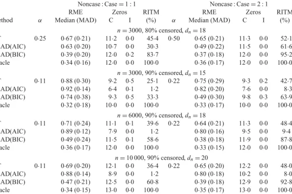
Table 1.Model selection performance in the scenario of a few large effects
Noncase : Case=1 : 1 Noncase : Case=2 : 1
RME Zeros RITM RME Zeros RITM
Method α Median (MAD) C I (%) α Median (MAD) C I (%)
n=3000, 80% censored,dn=18
HT 0·25 0·67 (0·21) 11·2 0·0 45·4 0·50 0·65 (0·21) 11·3 0·0 52·1 SCAD(AIC) 0·63 (0·20) 10·7 0·0 30·3 0·49 (0·22) 11·5 0·0 61·6 SCAD(BIC) 0·39 (0·20) 12·0 0·2 83·7 0·37 (0·18) 12·0 0·0 95·2 Oracle 0·34 (0·16) 12·0 0·0 100·0 0·36 (0·17) 12·0 0·0 100·0
n=3000, 90% censored,dn=15
HT 0·11 0·88 (0·30) 9·2 0·5 25·1 0·22 0·75 (0·29) 9·3 0·2 42·7 SCAD(AIC) 0·92 (0·14) 6·4 0·1 1·2 0·82 (0·20) 7·6 0·0 8·3 SCAD(BIC) 0·74 (0·38) 9·3 0·5 33·3 0·49 (0·30) 9·8 0·3 63·9 Oracle 0·32 (0·18) 10·0 0·0 100·0 0·33 (0·17) 10·0 0·0 100·0
n=6000, 90% censored,dn=18
HT 0·11 0·71 (0·24) 11·1 0·1 39·6 0·22 0·64 (0·21) 11·3 0·0 48·4 SCAD(AIC) 0·89 (0·12) 7·9 0·0 1·2 0·80 (0·16) 9·5 0·0 9·4 SCAD(BIC) 0·49 (0·24) 11·5 0·1 58·6 0·38 (0·18) 11·9 0·0 87·8 Oracle 0·36 (0·17) 12·0 0·0 100·0 0·33 (0·15) 12·0 0·0 100·0
n=10 000, 90% censored,dn=20
HT 0·11 0·69 (0·20) 12·1 0·0 36·4 0·22 0·65 (0·20) 12·2 0·0 48·0 SCAD(AIC) 0·88 (0·14) 8·9 0·0 1·2 0·80 (0·18) 10·2 0·0 8·0 SCAD(BIC) 0·47 (0·21) 12·5 0·0 60·8 0·39 (0·18) 12·9 0·0 92·8 Oracle 0·34 (0·15) 13·0 0·0 100·0 0·35 (0·17) 13·0 0·0 100·0 α, subcohort sampling probability; RME, relative model error; MAD, median absolute deviation; C, average number of zero parameters correctly identified as zero; I, average number of nonzero parameters incorrectly identified as zero; RITM, rate of identifying true model; HT, hard threshold; SCAD(AIC), smoothly clipped absolute deviation withλAIC
n ; SCAD(BIC), smoothly clipped absolute deviation withλBICn .
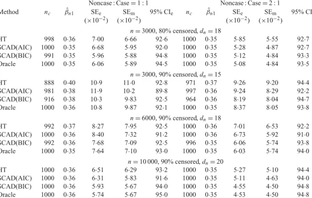
measures of variable selection performance, we also calculate the average number of parameters correctly estimated as zero, the average number of parameters erroneously estimated as zero, and the overall rate of identifying the true model. Point estimates, empirical and model-based standard errors, and empirical 95% confidence interval coverages are calculated forβn01=0·35
in the first scenario.
Table1summarizes the simulation results in the scenario of a few large effects. The penalized method with tuning parameterλBICn has by far the best performance in all settings in terms of the relative model error and the rate of identifying the true model. The inferior performance ofλAICn is apparently due to overfitting, as reflected by the low average number of correctly identified zero parameters; this is consistent with the theoretical findings ofWang et al.(2007) andZhang et al.
(2010). For bothλAICn andλBICn , more noncases in the case-cohort design and lower censoring rates are associated with better prediction and variable selection performance. Table2summarizes the parameter estimation results ofβn01=0·35 under the same settings as for Table1, but using only
simulation replications whereβn01is correctly identified as nonzero. Conditional onβˆn1 |=0, all
procedures produce approximately unbiased point and standard error estimates, with coverage close to the nominal level. The normality of the sampling distributions ofβˆn1was assessed by
Q-Q plots, shown in the Supplementary Material. The sampling distribution ofβˆn1is a mixture
Table 2.Estimation performance forβn01=0·35in the scenario of a few large effects; results are
based on replications whereβˆn1 |=0
Noncase : Case=1 : 1 Noncase : Case=2 : 1
Method nc βˆn1 SEe SEm 95% CIe nc βˆn1 SEe SEm 95% CIe
(×10−2) (×10−2) (×10−2) (×10−2)
n=3000, 80% censored,dn=18
HT 998 0·36 7·00 6·66 92·6 1000 0·35 5·85 5·55 92·7
SCAD(AIC) 1000 0·35 6·68 5·95 92·0 1000 0·35 5·28 4·87 92·7
SCAD(BIC) 991 0·35 5·96 5·88 94·8 1000 0·35 5·12 4·84 93·3
Oracle 1000 0·35 6·06 5·89 94·5 1000 0·35 5·08 4·84 93·5
n=3000, 90% censored,dn=15
HT 888 0·40 10·9 11·0 92·8 971 0·37 9·26 9·20 94·4
SCAD(AIC) 981 0·38 11·9 10·2 89·8 997 0·36 9·24 8·29 92·2
SCAD(BIC) 916 0·38 10·3 9·83 92·5 964 0·36 8·19 8·04 94·7
Oracle 1000 0·36 10·8 9·87 92·1 1000 0·35 8·37 8·05 93·8
n=6000, 90% censored,dn=18
HT 992 0·37 8·27 7·95 92·5 1000 0·36 7·01 6·53 92·2
SCAD(AIC) 1000 0·36 8·40 7·32 91·2 1000 0·36 6·73 5·92 91·0
SCAD(BIC) 992 0·36 7·68 7·09 92·5 996 0·35 6·06 5·74 93·8
Oracle 1000 0·35 7·64 7·10 93·0 1000 0·35 6·03 5·74 94·0
n=10 000, 90% censored,dn=20
HT 1000 0·36 6·51 6·29 93·2 1000 0·35 5·27 5·10 94·4
SCAD(AIC) 1000 0·36 6·31 5·83 91·6 1000 0·35 5·11 4·63 94·0 SCAD(BIC) 1000 0·36 5·93 5·67 94·0 1000 0·35 4·55 4·50 94·8
Oracle 1000 0·36 5·74 5·67 95·0 1000 0·35 4·53 4·50 94·8
nc, number of simulation replications whereβˆn1 |=0; SEe, empirical standard error; SEm, model-based standard error;
95% CIe, empirical 95% confidence interval coverage; HT, hard threshold; SCAD(AIC), smoothly clipped absolute
deviation withλnAIC; SCAD(BIC), smoothly clipped absolute deviation withλBICn .
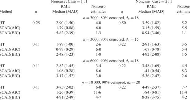
Table 3summarizes the simulation results in the scenario of many small effects, where all βn0=0·1. In this scenario the oracle model is just the unpenalized full model with the relative
model error being unity by definition, which is not very informative and hence not included in the table. With many small but nonzero effects, none of the three methods can identify all the effects with a high probability, as reflected by the near-zero rate of identifying the true model in all settings, which is not shown in the table. The inference results are not satisfactory either; they are not shown due to space limitations. Nevertheless, λAICn produces the smallest relative model error, suggesting that it has the best prediction performance among the three methods. Moreover,λAICn correctly identifies the largest number of small effects as nonzero. The Bayesian information criterion tends to select sparse models, so it may not perform as well as the Akaike information criterion when there are many small nonzero parameters. The relative model error is not comparable across different settings because it depends on the model error of the full model, which shows large variation in this scenario.
5·2. Analysis of the Busselton Health Study
Table 3.Model selection performance in the scenario of many small effects with allβn0=0·1
Noncase : Case=1 : 1 Noncase : Case=2 : 1
RME Nonzero RME Nonzero
Method α Median (MAD) estimates α Median (MAD) estimates
n=3000, 80% censored,dn=18
HT 0·25 2·90 (1·50) 4·0 0·50 3·59 (1·82) 5·2
SCAD(AIC) 1·79 (0·88) 6·0 3·15 (1·59) 5·5
SCAD(BIC) 5·62 (2·39) 1·3 8·94 (3·46) 1·1
n=3000, 90% censored,dn=15
HT 0·11 1·89 (1·00) 2·6 0·22 2·91 (1·63) 3·5
SCAD(AIC) 0·99 (0·29) 6·0 1·67 (0·78) 5·4
SCAD(BIC) 2·48 (1·23) 1·8 4·92 (2·08) 1·5
n=6000, 90% censored,dn=18
HT 0·11 2·82 (1·45) 3·4 0·22 3·48 (1·69) 4·5
SCAD(AIC) 1·08 (0·28) 8·6 1·41 (0·54) 8·3
SCAD(BIC) 3·17 (1·52) 3·0 5·36 (2·47) 2·6
n=10 000, 90% censored,dn=20
HT 0·11 3·85 (2·02) 6·0 0·22 4·49 (2·37) 7·7
SCAD(AIC) 1·26 (0·39) 11·6 1·84 (0·81) 11·4
SCAD(BIC) 4·91 (2·49) 4·7 8·38 (3·75) 4·2
α, subcohort sampling probability; RME, relative model error; MAD, median absolute deviation; Nonzero estimates, average number of parameters not estimated as zero; HT, hard threshold; SCAD(AIC), smoothly clipped absolute deviation withλAICn ; SCAD(BIC), smoothly clipped absolute deviation withλnBIC.
risk factors in the variable selection process: age, body mass index, blood pressure treatment, systolic blood pressure, cholesterol, triglycerides, haemoglobin and smoking status. All variables were measured at baseline. The full cohort of this analysis consists of 1401 subjects aged 40 to 89 years who participated in the Busselton Health Survey in 1981 and had no history of diagnosed coronary heart disease or stroke at that time. Subjects were followed until 31 December 1998, and their time to stroke, if one took place, was recorded. Subjects were treated as censored if they left Western Australia during the follow-up period. There were 118 incidences of stroke in the full cohort during the follow-up period. To reduce costs and preserve stored serum, a case-cohort design was used where the serum ferritin level was measured for only a randomly selected subcohort plus all stroke cases. The size of the random subcohort was 450, and the case-cohort size was 513.
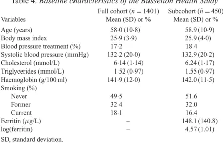
Table4summarizes the baseline characteristics of the full cohort and subcohort. The average ferritin level is not available for the full cohort due to the case-cohort design. The summary statis-tics for the baseline characterisstatis-tics of the full cohort and the subcohort are similar, suggesting that the subcohort is representative of the full cohort.
We apply the hard-threshold method and the penalized variable selection procedures with tun-ing parametersλAICn andλnBICto the Busselton Health Study. In order to avoid missing any poten-tially important effects, we also include in the initial model the quadratic terms of all continuous covariates as well as interactions between ferritin and all covariates. The total number of param-eters is 28. All continuous covariates are standardized using the means and standard deviations from the subcohort, shown in Table4. To decrease their skewness, we log-transformed the val-ues of ferritin and triglycerides before standardization. The tuning parameter selector identifies λAIC
n =0·244 andλBICn =0·305. Table5shows the models identified by the three methods. Due to space limitations, only terms that are selected by at least one method are shown. The use of λAIC
Table 4.Baseline characteristics of the Busselton Health Study
Full cohort (n=1401) Subcohort (n˜=450)
Variables Mean (SD) or % Mean (SD) or %
Age (years) 58·0(10·8) 58.9 (10·9)
Body mass index 25·9(3·9) 25.9 (4·0)
Blood pressure treatment (%) 17·2 18.4
Systolic blood pressure (mmHg) 132·2(20·0) 132.9 (20·2) Cholesterol (mmol/L) 6·14(1·14) 6.24 (1·17) Triglycerides (mmol/L) 1·52(0·97) 1.55 (0·97) Haemoglobin (g/100 ml) 141·9(12·0) 142.0 (11·5) Smoking (%)
Never 49·5 51.6
Former 32·4 32.0
Current 18·1 16.4
Ferritin (μg/L) – 148.1 (140.8)
log(ferritin) – 4.57 (1.01)
SD, standard deviation.
Table 5.Estimated coefficients and standard errors for the Busselton Health Study data; all continuous covariates were standardized using the means and standard deviations based on
the random subcohort before applying the variable selection procedure
Hard threshold SCAD(AIC) SCAD(BIC)
Variable β(ˆ SEˆ) β(ˆ SEˆ ) β(ˆ SEˆ)
Age (years) 0.92 (0·27) 0·87(0·15) 0.85 (0·14)
Sex (1=female) 0 (–) −0·61(0·26) −0.65 (0·25)
Blood pressure treatment 0.83 (0.34) 0·83(0.29) 0.89 (0·25)
Systolic blood pressure 0 (–) 0·21(0·15) 0 (–)
Systolic blood pressure2 0 (–) 0·092(0.067) 0.16 (0·044)
log(triglycerides) 0 (–) −0·24(0·18) 0 (–)
log2(triglycerides) 0 (–) 0·18(0·093) 0 (–)
SCAD(AIC), smoothly clipped absolute deviation withλAIC
n ; SCAD(BIC), smoothly clipped absolute deviation withλBICn .
important risk factors for stroke. The procedure usingλnAIC additionally selects the linear term of systolic blood pressure and the linear and squared terms of triglycerides. The hard-threshold method selects only age and blood pressure treatment.
To shed some light on which model provides the best fit to the data, we performed five-fold crossvalidation. The average log-pseudo-partial likelihood from the test datasets is used as the validation statistic. The hard-threshold method and penalized variable selection withλAICn andλnBIC give validation statistics of−621·5,−627·7 and−614·0, respectively. Therefore, we consider the model withλBICn to be the best fit to the Busselton data. According to this model, increased age, maleness, blood pressure treatment, and increased systolic blood pressure are associated with a higher risk of stroke. There is no evidence that serum ferritin level is associated with stroke.
6. DISCUSSION
in Table2, it is reasonable to assume that the maximizer identified by using the unpenalized esti-mator as the initial value is the(n/dn)1/2-consistent local maximizer described in Theorems1
and2.
In this paper the quantityα(ˆ t) used in the weight functionρ(t)is calculated at each failure time-point and so is time-dependent. When cases are rare,α(ˆ t)is almost constant acrosst. How-ever, using time-dependentα(ˆ t)is more general and allows the sampling probability to vary with time. Therefore, we useα(ˆ t)in this paper. A potential practical issue is thatα(ˆ t)may not be reli-able if the number of noncases in the random subcohort is very small, although this is highly unlikely due to the use of case-cohort design for studies of rare disease. In the unlikely situation where there is no noncase left in the subcohort, α(ˆ t) is not well-defined. To avoid computa-tional difficulties, one can define(1−)ξ/α(ˆ t)=0 ifα(ˆ t)=0. In fact, whenα(ˆ t)=0, 1− is necessarily zero for all subjects remaining in the subcohort.
There is a strong line of research on the convergence of and post-selection inference for penal-ized estimators (Leeb & P¨otscher, 2005;Leeb & P¨otscher,2006;P¨otscher & Leeb,2009). In particular,P¨otscher & Leeb(2009) showed that the penalized estimators are not uniformly con-sistent, and that their asymptotic distributions are nonnormal if the true parameter lies within a shrinking neighbourhood of zero with rate(dn/n)1/2. The lack of local regularity is a theoretical limitation of penalized variable selection methods. However, in this paper Condition5, together with the requirement thatλn j(n/dn)1/2→ ∞for all j, ensures that the nonzero parameters are uniformly larger than O{(dn/n)1/2}, hence avoiding the aforementioned irregularity. Our sim-ulation study suggests that the performance of the proposed variable selection method depends on the true effect size. In practice, since this size is unknown, we suggest conducting penalized variable selection with both Akaike and Bayesian information criteria-based tuning parameter selection, and then using crossvalidation to choose the best model, as done in§5·2. Theoretical justification of these model selection approaches will be investigated further. Moreover, as the regularity conditions required for our asymptotic results may not be testable in finite samples, it will be important to replicate findings from one particular finite data analysis. One possible way to examine the consistency of findings is to use bootstrap data or to apply a resampling-based variable selection approach such as stability selection (Meinshausen & B¨uhlmann,2010).
In the Busselton data analysis we standardized all continuous covariates, for several rea-sons. First, this makes the regression coefficients comparable. Second, it reduces the correla-tion between the linear and quadratic terms and between the main effect and interaccorrela-tion terms, which generally results in more robust and precise parameter estimates. More importantly, penal-ized regression procedures are not invariant with respect to covariate scaling, and standardization makes the penalization fair for all covariates (Tibshirani,1997). For these reasons, we recommend standardizing continuous covariates before carrying out penalized regression.
ACKNOWLEDGEMENT
We thank Professor Matthew Knuiman and the Busselton Population Medical Research Foun-dation for permission to use the data in the analysis of§5·2. This work was partially supported by the U.S. National Institutes of Health.
SUPPLEMENTARY MATERIAL
Supplementary material available atBiometrikaonline includes the proofs of the lemmas in the Appendix, the estimation of the covariance matrix n(βn0), and Q-Q plots of the estimate
ˆ
APPENDIX
Proofs of the theorems
Throughout the proofs, we write ˜n(βn0)j=∂˜n(βn0)/∂βn j, ˜n(βn0)j k=∂2˜n(βn0)/(∂βn j∂βnk) and
˜
n(βn0)j kl=∂3˜n(βn0)/(∂βn j∂βnk∂βnl). We also letV˜n j k(βn0,t),Vn j k(βn0,t),S˜n j k(2)(βn0,t)andS(n j k2)(βn0,t) be the (j,k)th components of the corresponding matrices. For a matrix A= {ai j}(i,j=1, . . . ,n), the
norm is defined asA =(ni=1
n j=1a
2
i j)
1/2
. The following lemma will be used repeatedly.
LEMMAA1. Let Wn(t) and Gn(t) be two sequences of processes with bounded variation almost
surely, and suppose that Gn(t)is progressively measurable and cadlag. For some constantτ, assume
thatsup0tτWn(t)−W(t) →0in probability for some bounded process W(t), that Wn(t)is
mono-tone on [0, τ], and that Gn(t)converges to a zero-mean process with continuous sample paths in the
metric spaceBV[0, τ], the bounded variation function space on[0, τ]. Then bothsup0tτ t
0{Wn(s)−
W(s)}dGn(s)andsup0tτ t
0Gn(s)d{Wn(s)−W(s)}converge to zero in probability as n→ ∞.
The proof of this lemma follows straightforwardly from that of Lemma 1 inLin(2000), upon noting that a process with bounded variation can be decomposed into two monotone processes.
We also need the following lemmas, proofs of which are provided in the Supplementary Material.
LEMMAA2. Letξ=(ξ1, . . . , ξn)be a random vector containingn ones and n˜ − ˜n zeros, with each
permutation equally likely. Let Xni(t) (i=1, . . . ,n)be a triangular array of real-valued random processes
on[0, τ], with E{Xni(t)} =μn(t),var{Xni(0)}<∞andvar{Xni(τ)}<∞for all i and n. Let Xn(t)=
{Xn1(t), . . . ,Xnn(t)}andξ be independent. Suppose that almost all paths of Xni(t)have finite variation.
Then n−1/2n
i=1ξi{Xni(t)−μn(t)}converges weakly to a tight zero-mean Gaussian process and hence
n−1n
i=1ξi{Xni(t)−μn(t)}converges in probability to zero uniformly in t.
LEMMAA3. Given thatξ is independent ofand Y(t), n1/2{ ˆα−1(t)−α−1}converges weakly to a
zero-mean Gaussian process.
LEMMAA4. Under Conditions 1–3, for any nonzero dn×1 constant vector un with un =
C<∞ and un0=cn>0, where ·0 denotes the number of nonzero components of a vector,
n1/2{ ˜S(0)
n (βn0,t)−Sn(0)(βn0,t)}, (n/cn)1/2uTn{ ˜S(
1)
n (βn0,t)−Sn(1)(βn0,t)} and n1/2c−n1u T n{ ˜S(
2)
n (βn0,t)−
S(2)
n (βn0,t)}unall converge weakly to tight zero-mean Gaussian processes.
LEMMAA5. Under Conditions 1–4, for any nonzero dn×1 constant vector un with un =1,
n−1/2uT n−
1/2
n (βn0)˜n(βn0)converges to a standard normal distribution, wheren(βn0)is the covariance
matrix of n−1/2˜
n(βn0).
LEMMAA6. Under Conditions 1–4, n−1/2{ ˜
n(βn0)j k+n In(βn0)j k} is Op(1) for j,k=1, . . . ,dn,
where In(βn0)j kis the(j,k)th component of In(βn0)as defined in§3·2.
LEMMAA7. Under Conditions1–6, if dn4/n→0,λn j→0and λn jn1/2dn−1/2→ ∞with probability
tending to1, for any givenβn,Isatisfyingβn,I−βn0,I =O(dn1/2n−
1/2)
and any constant C, we have that ˜
Qn{(βnT,I,0T)T} =maxβn,IICdn1/2n−1/2Q˜n{(β T
n,I, βnT,II)T}.
Proof of Theorem1. Letβn0be the true parameters, and letαn=dn1/2(n−1/2+an). It suffices to show
that for any ε >0 and any constant vectorun withun =C, there exists a large enough C such that
such that ˆβn−βn0 =Op(αn). SincePλn j(0)=0 andPλn j(·)0, we have
˜
Qn(βn0+αnun)− ˜Qn(βn0)
{ ˜n(βn0+αnun)− ˜n(βn0)} −n
kn
j=1
{Pλn j(|βn0j+αnun j|)−Pλn j(|βn0j|)} =I1−I2.
We first considerI1. By Taylor expansion,
I1=αnuTn˜n(βn0)+ 1 2α
2
nu T
n˜n(βn0)un+
1 6α 3 n n
i=1
dn
j,k,l=1 ˜
i (βn∗)j klun junkunl=I11+I12+I13,
where βn∗ lies between βn0 and βn0+αnun. From Lemma A5 we have ˜n(βn0)j=Op(n1/2) for
j=1, . . . ,dn. Therefore,
|I11| = |αnuTn˜n(βn0)|αnun ˜n(βn0) =αnunOp{(dnn)1/2} = unOp(αn2n).
The term I12 can be written as α2nuTn{ ˜n(βn0)+n In(βn0)}un/2−αn2uTnn In(βn0)un/2=J1−J2. By the Cauchy–Schwarz inequality, the fact that ˜n(βn0)j k+n In(βn0)j k=Op(n1/2) for j,k=1, . . . ,dn and
LemmaA6, we have|J1|αn2un2 ˜n(βn0)+n In(βn0)/2= un2Op(α2nn
1/2
dn)= un2op(α2nn). By
spectral decomposition of In(βn0)and Condition4,|J2|αn2un2nλmin{In(βn0)}/2un2(αn2n)C2/2. Under Conditions 1–3, ∂V˜n j k(βn∗,t)/∂βnl has bounded variation in t for i=1, . . . ,n and
j,k,l=1, . . . ,dn. Therefore ˜i(βn∗)j kl= − τ
0 ∂V˜n j k(βn∗,t)/∂βnldNi(t) is Op(1). Combining this with αn=dn1/2(n−
1/2+
an), dn4/n→0 and d
2
nan→0, we obtain |I13| =Op(dn3/2)nα
3
nun3=
Op{dn2(n−
1/2+
an)}nαn2un3= un3op(α2nn). Therefore, for large enoughun, |J2| dominates|I11|, |J1|and|I13|.
Now considerI2. By Taylor expansion and the Cauchy–Schwarz inequality,
|I2| =
n
kn
j=1
Pλn j (|βn0j|)sgn(βn0j)αnun j+
1 2n
kn
j=1
Pλn j (|βn0j|)α2nu
2
n j{1+o(1)} n kn
j=1
Pλn j (|βn0j|)αnun j +12n
kn
j=1
Pλn j (|βn0j|)αn2u
2
n j{1+o(1)}
nαnank1n/2un +
1 2nα
2
nbnun2{1+o(1)}
= unOp(αn2n).
The last equality holds becausean=Op(αndn−1/2)andbn→0 under Condition5. Therefore,|J2| domi-nates|I2|for large enoughC. SinceJ2is negative, it follows that for large enoughC, Q˜n(βn0+αnun)−
˜
Qn(βn0)is negative with probability tending to 1 asn→ ∞. This completes the proof of Theorem1.
Proof of Theorem2. The assertion that βˆn,II=0 with probability tending to 1 as n→ ∞ follows directly from LemmaA7. To prove the second assertion, we first show that
n1/2uT n−
1/2
n11
(In11+n)(βˆn,I−βn0,I){1+op(1)} +Bn
=n−1/2uT n−
1/2
n11 ˜n1(βn0)+op(1), (A1)
fact thatβˆn,II−βn0,II=0 with probability tending to 1, we have ˜
n1(βn0)+ ˜n1(βn0)(βˆn,I−βn0,I)+(βˆn,I−βn0,I)T˜n1(βn∗)(βˆn,I−βn0,I)/2
−n Bn−n∗∗n (βˆn,I−βn0,I)=0 (A2)
with probability tending to 1, where˜n1(βn0)consists of the firstkn×kncomponents of˜n(βn0),˜n1(βn∗)
consists of the firstkn×kn×kncomponents of˜n(βn∗),βn∗lies betweenβˆnandβn0, andn∗∗=n(βn∗∗)
withβn∗∗betweenβˆnandβn0. Upon rearranging (A2), we get
{ ˜
n1(βn0)−nn∗∗}(βˆn,I−βn0,I)−n Bn= − ˜n1(βn0)− 1
2(βˆn,I−βn0,I)
T˜
n1(βn∗)(βˆn,I−βn0,I). (A3)
Writeνn=(βˆn,I−βn0,I)T˜n1(βn∗)(βˆn,I−βn0,I). Multiplying both sides of (A3) byn−1/2uTn−
1/2
n11 gives
n1/2uT n−
1/2
n11
1
n˜
n1(βn0)−n∗∗
(βˆn,I−βn0,I)−n1/2uTn−
1/2
n11 Bn
= −n−1/2uT n−
1/2
n11 ˜n1(βn0)−n−1/2uTn−
1/2
n11 νn/2. (A4)
By the Cauchy–Schwarz inequality,νn ˆβn,I−βn0,I2
n i=1{
kn
j,k,l=1˜i1(β∗) 2
j kl}
1/2. As shown in the
proof of Theorem1,˜i1(β∗)j kl=Op(1), soνn =Op{(dn/n)nkn3/2} =Op(dn5/2). By spectral
decomposi-tion ofn−111/2,dn5/n→0 and Condition4, we have
1 2n
−1/2
uT n−
1/2
n11 νn
unνn
2 n
−1/2λ
max(n−1/2)=Op(dn5/2n−
1/2)=
op(1). (A5)
The inequality in (A5) holds by the Cauchy–Schwarz inequality and the Cauchy
inter-lacing inequality for symmetric matrices. Moreover, uT
n
−1/2
n11 n−1˜n1(βn0)(βˆn,I−βn0,I)=
uT n−
1/2
n11 {n− 1˜
n1(βn0)+In11(βn0)}(βˆn,I−βn0,I)−uTn−
1/2
n11 In11(βn0)(βˆn,I−βn0,I)=J1−J2. By the Cauchy–Schwarz inequality and LemmaA6,|J1|uTn−
1/2
n11 n−1˜n1(βn0)+In11(βn0) ˆβn,I−βn0,I = uT
n−
1/2
n11 ˆβn,I−βn0,IOp(dnn−1/2). Also, we have |J2|uTn−
1/2
n11 ˆβn,I−βn0,Iλmin(In11) uT
n−
1/2
n11 ˆβn,I−βn0,Iλmin(In). Then, by Condition4,
J1
J2
uTn−
1/2
n11 ˆβn,I−βn0,IOp(dnn−1/2)
uT n
−1/2
n11 ˆβn,I−βn0,Iλmin(In)
=Op(dnn−1/2)=op(1).
Therefore J1=op(J2) and uTn−
1/2
n11 n−1˜n1(βn0)(βˆn,I−βn0,I)= −uTn−
1/2
n11 In11(βn0)(βˆn,I−
βn0,I){1+op(1)}. Sinceβˆnconverges toβn0in probability, it follows that
uT n
−1/2
n11
1
n˜
n1(βn0)−n∗∗
(βˆn,I−βn0,I)= −uTn
−1/2
n11
In11(βn0)+n
(βˆn,I−βn0,I){1+op(1)}. (A6) By (A4), (A5) and (A6), we have that (A1) holds. By LemmaA5,n−1/2uT
n
−1/2
n11 ˜n1(βn0)converges to the standard normal distribution. Therefore,n1/2uT
n−
1/2
n11 (In11+n){ ˆβn,I−βn0,I+(In11+n)−1Bn} →
N(0,1)in distribution. This proves the second assertion of Theorem2.
REFERENCES
AKAIKE, H. (1973). Maximum likelihood identification of Gaussian autoregressive moving average models.
Biometrika60, 255–65.
BARLOW, W. E. (1994). Robust variance estimation for the case-cohort design.Biometrics50, 1064–72.
BORGAN, O.,LANGHOLZ, B.,SAMUELSEN, S. O.,GOLDSTEIN, L. &POGODA, J. (2000). Exposure stratified case-cohort
designs.Lifetime Data Anal.6, 39–58.
CHO, H. &QU, A. (2013). Model selection for correlated data with diverging number of parameters.Statist. Sinica
23, 901–27.
COX, D. R. (1972). Regression models and life-tables (with Discussion).J. R. Statist. Soc.B34, 187–220.
CRAVEN, P. &WAHBA, G. (1979). Smoothing noisy data with spline functions: Estimating the correct degree of
smooth-ing by the method of generalized cross-validation.Numer. Math.31, 377–403.
CULLEN, K. J. (1972). Mass health examinations in the Busselton population, 1966 to 1970.Austr. J. Med.2, 714–8.
FAN, J. &LI, R. (2001). Variable selection via nonconcave penalized likelihood and its oracle properties.J. Am. Statist. Assoc.96, 1348–60.
FAN, J. &LI, R. (2002). Variable selection for Cox’s proportional hazards model and frailty model.Ann. Statist.30, 74–99.
FAN, Y. &TANG, C. Y. (2013). Tuning parameter selection in high dimensional penalized likelihood.J. R. Statist. Soc.
B75, 531–52.
HASTIE, T.,TIBSHIRANI, R. J. &FRIEDMAN, J. (2009).The Elements of Statistical Learning. Berlin: Springer, 2nd ed.
HUBER, P. J. (1973). Robust regression: Asymptotics, conjectures, and Monte Carlo.Ann. Statist.1, 799–821.
HUNTER, D. &LI, R. (2005). Variable selection using MM algorithms.Ann. Statist.33, 1617–42.
KALBFLEISCH, J. D. &LAWLESS, J. F. (1988). Likelihood analysis of multi-state models for disease incidence and
mortality.Statist. Med.7, 149–60.
KANG, S. &CAI, J. (2009). Marginal hazards model for case-cohort studies with multiple disease outcomes.Biometrika
96, 887–901.
KIM, S.,CAI, J. &LU, W. (2013). More efficient estimators for case-cohort studies.Biometrika100, 695–708.
KNUIMAN, M. W.,DIVITINI, M. L.,OLYNYK, J. K.,CULLEN, D. J. &BARTHOLOMEW, H. C. (2003). Serum ferritin and
cardiovascular disease: A 17-year follow-up study in Busselton, Western Australia.Am. J. Epidemiol.158, 144–9.
KULICH, M. &LIN, D. (2004). Improving the efficiency of relative-risk estimation in case-cohort studies.J. Am. Statist.
Assoc.99, 832–44.
LEEB, H. &P¨OTSCHER, B. M. (2005). Model selection and inference: Facts and fiction.Economet. Theory21, 21–59. LEEB, H. &P¨OTSCHER, B. M. (2006). Can one estimate the conditional distribution of post-model-selection estimators?
Ann. Statist.34, 2554–91.
LIN, D. (2000). On fitting Cox’s proportional hazards models to survey data.Biometrika87, 37–47.
MEINSHAUSEN, N. &B¨UHLMANN, P. (2010). Stability selection (with Discussion).J. R. Statist. Soc.B72, 417–73.
PENG, H. &FAN, J. (2004). Nonconcave penalized likelihood with a diverging number of parameters.Ann. Statist.32, 928–61.
PORTNOY, S. (1988). Asymptotic behavior of likelihood methods for exponential families when the number of
param-eters tends to infinity.Ann. Statist.16, 356–66.
P¨OTSCHER, B. M. &LEEB, H. (2009). On the distribution of penalized maximum likelihood estimators: The LASSO,
SCAD, and thresholding.J. Mult. Anal.100, 2065–82.
PRENTICE, R. L. (1986). A case-cohort design for epidemiologic cohort studies and disease prevention trials.
Biometrika73, 1–11.
SCHWARZ, G. (1978). Estimating the dimension of a model.Ann. Statist.6, 461–4.
SELF, S. G. &PRENTICE, R. L. (1988). Asymptotic distribution theory and efficiency results for case-cohort studies.
Ann. Statist.16, 64–81.
TIBSHIRANI, R. J. (1996). Regression shrinkage and selection via the lasso.J. R. Statist. Soc.B58, 267–88.
TIBSHIRANI, R. J. (1997). The lasso method for variable selection in the Cox model.Statist. Med.16, 385–95.
WANG, H.,LI, B. &LENG, C. (2009). Shrinkage tuning parameter selection with a diverging number of parameters.
J. R. Statist. Soc.B71, 671–83.
WANG, H.,LI, R. &TSAI, C.-L. (2007). Tuning parameter selectors for the smoothly clipped absolute deviation method.
Biometrika94, 553–68.
ZHANG, C.-H. (2010). Nearly unbiased variable selection under minimax concave penalty.Ann. Statist.38, 894–942. ZHANG, Y.,LI, R. &TSAI, C.-L. (2010). Regularization parameter selections via generalized information criterion.
J. Am. Statist. Assoc.105, 312–23.
ZOU, H. (2006). The adaptive lasso and its oracle properties.J. Am. Statist. Assoc.101, 1418–29.
ZOU, H. &ZHANG, H. H. (2009). On the adaptive elastic-net with a diverging number of parameters.Ann. Statist.37, 1733–51.