205 |
P a g e
PERFORMANCE OF DYNAMIC SOURCE ROUTING
PROTOCOL FOR FIXED AND VARIABLE POWER
TRANSMISSIONS IN WIRELESS SENSOR NETWORK
N.Divya
1, U.Hari
21
PG Scholar, Embedded System Technology, Department of ECE, SRM University (India)
2
Asst. Prof, Department of ECE, SRM University (India)
ABSTRACT
A wireless sensor network consists of collection of sensor nodes deployed over a geographical area for
monitoring different parameters. The power source of sensor node consists of a battery with a limited energy
and it is impossible to recharge the battery, because nodes may be deployed in an unmanned or remote area.
Most of the power is consumed by the radio communication involved in the sensor network. So an energy
efficient communication scheme has to be designed to improve the network lifetime. DSR protocol is a reactive
protocol that makes it possible for all the nodes to find a route to a destination in a multiple network hops
dynamically. The network lifetime reduces by forwarding data with more transmission power. The intermediate
nodes spend more energy to transmit its own data and forward other nodes data. Therefore the intermediate
node drains out of energy soon. To solve this problem the transmission power has to adjusted for different
transmissions in the network according to distance towards the destination. The simulation is done using
TOSSIM simulator tool.
Keywords:
DSR (Dynamic Source Routing) Protocol, Intermediate Nodes, Network Lifetime,
Transmission power level, WSN (Wireless Sensor Network
I. INTRODUCTION
Wireless sensor network (WSN) is the collection of sensor nodes that performs a given task with coordination
and in-network processing. These nodes have the potential of sensing, processing and communication of data
with each other wirelessly. The basic task of sensor networks is to sense the events, collect data and send it to
their destination. On the other hand, WSNs are power constrained distributed systems with low energy, low
bandwidth and shorter communication range.
206 |
P a g e
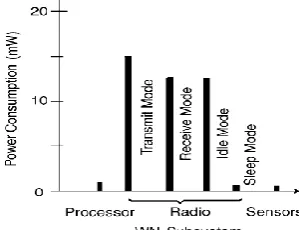
Sensor networks require sensing systems that are long-lived and environmentally resilient. Power consumptionneeds to be taken into account as a design constraint. Out of all functions in a sensor node, the radio
communication draws most of the energy as shown in Figure 1.
The wireless sensor node has a constrained power source and replenishment of power may be limited or
impossible altogether. In this work micaz motes are considered. Battery operation for sensors used in
commercial applications is typically based on two AA alkaline cells or one Li-AA cell. Power management and
power conservation are critical functions for sensor networks, and one needs to design energy efficient protocols
and algorithms. The function of a sensor node in a sensor field is to detect events, perform local data processing,
and transmit processed data. Power consumption can therefore be allocated to three functional domains: sensing,
communication, and data processing, each of which requires optimization. In the context of communications, in
a multi hop sensor network a node may play the dual role of data collection and processing and of being a data
relay point. Most of the power is consumed by the radio communication. So an energy efficient communication
scheme has to be designed to improve the network lifetime.
II. RELATED WORK
M. N. Jambli and et al [1] evaluated the capability of AODV on how far it can react to network topology change
in Mobile WSN. They investigated the performance metrics namely packet loss and energy consumption of
mobile nodes with various speed, density and route update interval (RUI), for 9 nodes in (100×100) m2 network.
The presented results showed a high percentage of packet loss and the reduction in total network energy
consumption of mobile nodes if RUI is getting longer due to serious broken link caused by nodes movement.
Ali Abdul-Majed Ihbeel and Hasein Issa Sigiuk [2] made an attempt to evaluate the performance of DSR
routing protocol using some simulation network models, to investigate how well this protocol performs on
WSNs, in static and mobile environments, using NS-2 simulator. The performance study will focus on the
impact of the network size, network density (up to 450 nodes), and the number of sources (data connections).
The performance metrics used in this work are average end-to-end delay, packet delivery fraction, routing
overheads, and average energy consumption per delivered packet.
III. DYNAMIC SOURCE ROUTING PROTOCOL (DSR)
One of the reactive protocols is dynamic source routing protocol. This protocol makes it possible for all the
nodes to find a route to a destination in a multiple network hops dynamically. The distinguishing features of
DSR are: low network overhead, no extra infrastructure for administration and the use of source routing. Source
routing implies that the sender had full knowledge of the complete hop-by-hop route information to the
destination. The protocol is composed of the two main mechanisms of Route Discovery and Route Maintenance.
Normally routes are stored in a route cache of each node. When a node likes to communicate to a destination,
first it checks for the route for that particular destination in the route cache. If yes, the packets are sent with
source route header information to the destination. In the other case, if the route is not available at the route
cache; then the node will initiate the route discovery mechanism to get the route first [2].
The route discovery mechanism will flood the network with route request (RREQ) packets, and then the
neighbors will receive RREQ packets and check for the route to destination in their route cache. If the route is
207 |
P a g e
packet. Since RREQ and RREP packets both are source routed, original source can obtain the route and add toits route cache. In any case the link on a source route is broken; the source node is notified with a route error
(RERR) packet. Once the RERR is received, the source removes the route from its cache and route discovery
process is reinitiated.
DSR being a reactive routing protocol has no need to periodically flood the network for updating the routing
tables like table-driven routing protocols do. Intermediate nodes are able to utilize the route cache information
efficiently to reduce the control overhead.
DSR minimizes the overall network bandwidth overhead because of the fact that it does not use periodic routing
messages. By doing so DSR saves battery power as well as avoidance of routing updates that are large enough.
However there is a support from the MAC layer that informs the routing protocol of any failure in nodes in
DSR. In DSR protocol the forwarding nodes do not save the up-to date routing information, thus DSR takes the
use of source routing. DSR describes a flow id option that allows packets to be transmitted on a hop-by-hop
basis. This protocol is based on source routing where all the routing information is maintained at mobile nodes.
It has two major phases, which are Route Discovery and Route Maintenance. Route Reply would be created
only if the message has reached the correct destination node.
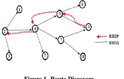
All the known routes are stored in the cache by DSR. When a node wants to send data to another node, it first
broadcasts an RREQ as shown in Figure 1. This RREQ is received by other nodes and as they receive it they
start searching their cache for any available route to the destination node. In case on any unavailable routes this
RREQ is forwarded while the address of the current node is being recorded in the hop sequence.
The RREQ propagates in the network until the availability of a route to the destination or the availability of the
destination itself. When this happens an RREP is generated and unicasted to the source node. The contents of
this RREP packet are the sequence of hops in the network for reaching the destination node. In the discovery of
an invalid route an error packet is sent to the source node and once this error packet is received, the hop that has
error is removed from the cache of the host and all routes containing this erroneous hop are deleted.
Figure 1- Route Discovery
To make the best use of the limited energy available to the sensor nodes, and hence to enhance the network
lifetime, it is important to design modulation scheme, transmit power and hop distance parameters in the
network stack. To solve the problems of minimizing energy to send data and finding optimum energy-efficient
transmit distances, the concept of energy per bit metric is used [3].
This metric defines a way of comparing energy consumption, the energy per bit (EPB) metric as:
EPB= (BD + BP) (PT + αPR) T (1)
208 |
P a g e
BD is the average number of data bits and BP is the average number of preamble bits. The terms PT and PR aretransmit and receive power, respectively. The parameter α is determined by the MAC protocol and represents
the proportion of time spent in receive mode compared to the proportion of time spent in transmit mode. Finally,
T is the time to transmit a bit.
The energy consumed when sending a packet of m bits over one hop wireless link can be expressed as[13],
EL (m,d) = {ET (m,d) + PTTst + Eencode } + {ER (m) + PRTst + Edecode} (2)
ET is energy used by the transmitter circuitry and power amplifier, ER is energy used by the receiver circuitry,
PT is power consumption of the transmitter circuitry, PRis power consumption of the receiver circuitry, Tst is
startup time of the transceiver, Eencode is energy used to encode, Edecode is the energy used to decode.
Assuming a linear relationship for the energy spent per bit at the transmitter and receiver circuitry ET and ER can
be written as[13],
ET (m,d) = m ( eTC + eTAdα ) (3)
ER(m) = meRC (4)
eTC, eTA, and eRC are hardware dependent parameters and α is the path loss exponent whose value varies from 2
(for free space) to 4 (for multipath channel models). The effect of the transceiver startup time, Tst, will greatly
depend of the type of MAC protocol used[13]. To minimize power consumption it is desired to have the
transceiver in a sleep mode as much as possible however constantly turning on and off the transceiver also
consumes energy to bring it to readiness for transmission or reception. eTA can be expressed as,
eTA = (S/N)r (NFrx) (No) (BW) (4π / λ)α (5)
( Gant) ( ηamp ) ( Rbit )
Where,
(S/N)r = minimum required signal to noise ratio at the receiver’s demodulator for an acceptable Eb/N0
NFrx =receiver noise figure
N0 = thermal noise floor in a 1 Hertz bandwidth (Watts/Hz)
BW = channel noise bandwidth
λ = wavelength in meters
α = path loss exponent
Gant = antenna gain
ηamp = transmitter power efficiency
Rbit = raw bit rate in bits per second
IV. POWER SCENARIOS
There are two possible power scenarios
4.1. Variable Transmission Power
In this case the radio dynamically adjust its transmission power so that (S/N)r is fixed to guarantee a certain
level of Eb/N0at the receiver. The transmission energy per bit is given by[13],
209 |
P a g e
Since (S/N)r is fixed at the receiver this also means that the probability p of bit error is fixed to the same valuefor each link.
4.2. Fixed Transmission Power
In this case the radio uses a fixed power for all transmissions. This case is considered because several
commercial radio interfaces have a very limited capability for dynamic power adjustments[13]. In this case it is
fixed to a certain value (ETA) at the transmitter and the (S/N)r at the receiver will then be,
(S/N)r = (ETA ) / (ζ dα) (7)
Since for most practical deployments d is different for each link then (S/N)r will also be different for each link.
This translates on a different probability of bit error for wireless hop.
In this work a DSR protocol performance is studied and analyzed under variable and fixed transmission power.
According to the distance between two nodes the transmission power can be adjusted. Thereby we can reduce
the consumption of power. Evaluating DSR protocol under various transmission power outperforms the fixed
range transmission.
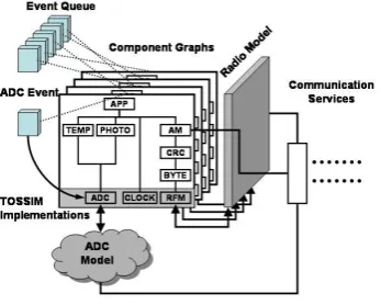
V. TOSSIM
TOSSIM captures the behavior and interactions of networks of thousands of TinyOS motes at network bit
granularity. Figure2 shows a graphical overview of TOSSIM.
Figure 2: TOSSIM Architecture: Frames, Events, Models,
Components, and ServicesThe TOSSIM architecture is composed of five parts: support for compiling TinyOS component graphs into the
simulation infrastructure, a discrete event queue, a small number of re-implemented TinyOS hardware
abstraction components, mechanisms for extensible radio and ADC models, and communication services for
external programs to interact with a simulation. TOSSIM takes advantage of TinyOS’s structure and whole
system compilation to generate discrete-event simulations directly from TinyOS component graphs. It runs the
same code that runs on sensor network hardware. By replacing a few low-level components (e.g., those shaded
in Figure 2), TOSSIM translates hardware interrupts into discrete simulator events; the simulator event queue
delivers the interrupts that drive the execution of a TinyOS application. The remainder of TinyOS code runs
unchanged. TOSSIM uses a very simple but surprisingly powerful abstraction for its wireless network. The
network is a directed graph, in which each vertex is a node, and each edge has a bit error probability [4]-[6].
Compiling to native code allows developers to use traditional tools such as debuggers in TOSSIM. As it is a
discrete event simulation, users can set debugger breakpoints and step through what is normally real-time code
210 |
P a g e
interact and monitor a running simulation; by keeping monitoring and interaction external to TOSSIM, the coresimulator engine remains very simple and efficient [7].
VI. POWERTOSSIM Z
Hardware power consumption has been incorporated into implementation of PowerTOSSIM z. Capturing the
power consumption of an application running on a given mote necessitates tracking of the behaviour of the
mote’s low level components, such as the microcontroller and the radio chip. An energy estimator must also
take into account the interfaces that TinyOS exports to manage them, and their support within TOSSIM.[11]
6.1 Tinyos Interfaces
The TinyOS 2.x power management interfaces are a major improvement over those implemented in TinyOS 1.x.
As stated in TEP 112 [8], TinyOS 1.x essentially relied on the application itself to handle the power on/power
off states of all the devices. This was accomplished through the use of the StdControl interface, which exports a
start and a stop command that any component can call over a given peripheral. This approach simplified the
design of PowerTOSSIM 1.x, since most of the calls could then be placed where this interface was
implemented, to gain a complete view of the mote’s power state. TinyOS 2.x operates differently in that it
divides the devices in two classes[11]:
1. The microcontroller, which fundamentally has enough information to independently calculate the power
stateto use.
2. The peripherals, which have simpler semantics (with the partial exception of the CC2420 Radio Chip, as we
will see later on) and two basic power states, on and off.
The relevant power management interfaces and their associated hardware are described in more detail
below.Only the devices relevant to our PowerTOSSIM z implementation will be analyzed, with particular
emphasis on TOSSIM support and its limitations. This description is at the heart of the design goals and
implementation of PowerTOSSIM z, and any future improvements.
6.2 Microcontroller Power Management: The Atm128 Mcu
The Atmega128 is a low-power CMOS 8-bit microcontroller based on the AVR enhanced RISC architecture [9].
It features six software selectable power-save states (shown in Table 1) which range from the IDLE state, which
stops the CPU while leaving all the other components active, down to the POWERDOWN state, which disables
all the components until the next interrupt or hardware reset. TinyOS exports one interface for the handling of
the microcontroller, which is called McuSleep, which exposes a single asynchronous command, sleep(), that is
called inside the TinyOS scheduler when the FIFO task queue is empty. The job of the sleep() command is to
calculate the correct power state in which to put the microcontroller. The task requires analysis of the state of
different registers[11].
Table 1: Atmega128 Power states
POWER STATE CURRENT
Active 8mA
Idle 4mA
211 |
P a g e
ADC Noise Reduction 1mAExtended Standby 160μA
Power-save 9μA
Power-down 0.3μA
RADIO CURRENT
Rx 7.03 mA
Tx (power = 00) 3.72 mA
Tx (power = 01) 5.21 mA
Tx (power = 03) 5.37 mA
Tx (power = 06) 6.47 mA
Tx (power = 09) 7.05 mA
Tx (power = 0F) 8.47 mA
Tx (power = 60) 11.57 mA
Tx (power = 80) 13.77 mA
Tx (power = C0) 17.37 mA
Tx (power = FF) 21.48 mA
This result is compared to the actual lowest possible state to which the MCU is allowed to go. Since some
external peripherals may require the MCU to not go below a given power state (for example if it will require the
CPU soonand the tradeoff between time spent in a low-power state and wake-up latency is not favorable),
TinyOS allows them to specify the lowest acceptable power state through the Mcu Power Override. Lowest
State() command. Despite first appearances, TOSSIM does not offer support for fine tracking of the behaviour
of the microcontroller. A port of the Mcu Sleep components exists, together with a representation of the
hardware registers as entries in a global array of uint8_t entries. However, these registers are never modified,
and the Mcu Sleep component itself is not wired inside the TOSSIM scheduler (which is missing a call to the
sleep() command when there are no tasks available). The power state of the microcontroller is of some
importance to our battery model: we assume that battery recovery can only take place with the MCU in
POWERSAVE or POWERDOWN modes. Therefore the TOSSIM scheduler is extended to call Mcu Sleep.
sleep() and we basic tracking of some of the components’ state is performed to allow Power TOSSIM 2 to report
meaningful values for the MCU state. The atm128 implementation also tracks the use of the LED and other
ports. LEDs are connected to Port G of the atm128 microcontroller, a 5 bit port. Bits 0, 1 and 2 are used to
directly manipulate the LED state, while bit 4 acts as a broadcast bit (controlling all the three LEDs at the same
time). The state of the SPI bus can be derived from the use of the flash and the radio stack (which both use the
SPIbus). TOSSIM uses the Simple Fcfs Arbiter to emulate the atm128 SPI bus (which allows some tracking of
the resources requiring and releasing the SPI bus)[11].
6.3 Peripheral Power Management
TinyOS 2.x divides the power management interfaces into two distinct classes, the microcontroller and the
peripherals. A richer set of interfaces (with respect to TinyOS 1.x) is offered for power management of
peripherals, described in TEP 115 [10] which can be categorized into two different models: explicit power
212 |
P a g e
memory components); simplistically, it can be understood as powering on or off a given device with the explicitpower management interface once the resource has been granted (in the case of the at45db interface, the SPI
bus). A more detailed description is available in [10].
VII. SIMULATION RESULTS
7.1 Energy Consumption
Figure 3 shows the energy consumption per delivered packet: This measure the energy expended per delivered
data packet.
Figure 3- Comparison of Energy Consumption
7.2 Throughput
It is the rate of successful message delivery over a communication channel as shown in Figure 4. Throughput is
measured in bits per second (bit/s or bps)
Figure 4- Comparison of Throughput
VIII. CONCLUSION
On comparing the performance of DSR protocol under fixed and variable power transmission is studied and
analyzed. Power transmissions when varied according to the number of hops in-between seems to be more
energy-efficient compared to fixed power transmission in wireless sensor network. Therefore the network
213 |
P a g e
REFERENCE
[1] M. N. Jambli, K. Zen, H. Lenando and A. Tully, “Performance Evaluation of AODV Routing Protocol
for Mobile Wireless Sensor Network,” 7th International Conference on IT in Asia (CITA), IEEE 2011.
[2] Ali Abdul-Majed Ihbeel 1 and Hasein Issa Sigiuk, “Performance Evaluation of Dynamic Source Routing
Protocol (DSR) on WSN” International Journal of Computing and Digital Systems, Int. J. Com. Dig.
Sys. 1, No. 1, 19-24 (2012)
[3] Ammer, J. and Rabaey, J. 2006. The energy-per-useful-bit metric for evaluating and optimizing sensor
network physical layers .In Proceedings of the IEEE International Workshop on Wireless Ad-hoc and
Sensor Networks. 695–700.
[4] TOSSIM: Accurate and Scalable Simulation of Entire TinyOS Applications Philip Levis, Nelson Lee,
Matt Welsh], and David Culler.
[5] D. Braginsky and D. Estrin. Rumor Routing Algorithm for Sensor Networks. In Proceedings of the First
ACM International Workshop on Wireless Sensor Networks and Applications, 2002.
[6] J. Elson, L. Girod, and D. Estrin. Fine-Grained Network Time Synchronization using Reference
Broadcasts. In Fifth Symposium on Operating Systems Design and Implementation (OSDI 2002),
Boston, MA, USA., dec 2002.
[7] D. Gay, P. Levis, R. von Behren, M. Welsh, E. Brewer, and D. Culler. The nesC Language: A Holistic
Approach to Networked Embedded Systems. In Proceedings of Programming Language Design and
Implementation (PLDI), June 2003.
[8] R. Szewczyk, P. Levis, M. Turon, L. Nachman, P. Buonadonna, and V. Handziski. Microcontroller
power management, Jan. 2007. Available at http://www.tinyos.net/tinyos-2.x/doc/html/ tep112.html.
[9] ATM128 datasheet, Jan. 2007. Available at http://www.siphec.com/microcontroller/
ATmega128(L)_complete.pdf.
[10] K. Klues, V. Handziski, J.-H. Hauer, and P. Levis. Power management of non-virtualized
devices.Available at http://www.tinyos.net/tinyos-2.x/doc/txt/ tep115.txt.
[11] Enrico Perla Art Ó Catháin Ricardo Simon Carbajo Meriel Huggard Ciarán Mc Goldrick
“PowerTOSSIM z: Realistic Energy Modelling for Wireless Sensor Network Environments”.
[12] Matthew Holland, TianqiWang, Bulent Tavli, Alireza Seyedi and Wendi Heinzelman “ Optimizing
Physical Layer Parameters for Wireless Sensor Networks” ACM Journal Name, Vol. , No. , 2009.