NORMALITY AND DATA TRANSFORMATION FOR APPLIED STATISTICAL ANALYSIS

United Kingdom

Vol. II, Issue 7, 2014

Licensed under Creative Common Page 1

NORMALITY AND DATA TRANSFORMATION FOR APPLIED STATISTICAL ANALYSIS

Singh, Ajay S.

Department of AEM, Faculty of Agriculture, University of Swaziland, Luyengo, Swaziland

[email protected]

Masuku, Micah B.

Department of AEM, Faculty of Agriculture, University of Swaziland, Luyengo, Swaziland

[email protected]

Abstract

Applications of statistical techniques are common in scientific and multidisciplinary research.

Statistical tools are useful to describe the numerical facts as well as relationship between the

factors and to test the independence of attributes or variables. Some researchers use statistics

to explain the findings of a phenomenon. However some other researchers use statistical tools

without understanding of the statistical technicality. Statistical errors are very common in

scientific research and 50 percent of the published articles have at least some error. These

errors are mainly about the important assumption of normality. The concept of normality and

data transformation are the most important part when using statistical techniques. The

assumption of normality is required for most of the statistical tools, namely correlation,

regression and parametric test because their validity is based on normality. Data

transformations are commonly used tools that can serve many functions in quantitative data

analysis. The main purpose of this paper is to highlight the basic and important assumption

based on normal distribution in terms normality test. The paper describes the concept of

normality and how to test the normality of data. In this paper also describes the tools for

normality in terms of standardized data transformation.

Keywords: Applied Statistical Analysis, Normal Distribution, Normality Test, Data

Licensed under Creative Common Page 2

INTRODUCTION

Applied statistical methods are commonly used in multidisciplinary research. Some of the

researchers use statistical tools without understanding their pre- requisites. Statistical errors are

very common in scientific research and at least one error in the 50% of research article

(Ghasemi and Zahedisal, 2012). Many of the statistical methods including correlation,

regression, analysis of variance and parametric tests are based on normal distribution. In other

words testing of normality is required for most of the statistical procedures. In the context of

correlation, regression and parametric test based on the normal distribution under the

assumption that the population from which the samples are taken is normally distributed (Altman

and Bland, 1995; Driscoll et al. 2000). Assumptions on statistical tools and important

assumption about the normality should be taken seriously; otherwise it is difficult to draw the

accurate and reliable conclusion about the reality (Royston, 1991; Oztuna et al. 2006).

BASICS OF NORMAL DISTRIBUTION

In the theory of probability, the normal distribution is commonly used for continuous probability

distribution functions. Normal distributions are also important in statistics and social sciences for

real-valued random variables whose distributions are not known (Casella and Berger, 2002;

Driscoll et al., 2000).

Normal distribution is useful because of the central limit theorem, which states that,

under mild conditions, the mean of many random variables independently drawn from the same

distribution is distributed approximately normal, irrespective of the form of the original

distribution. Physical quantities are expected to be the sum of many independent processes

and a distribution very close to the normal. Moreover, many results and methods can be derived

analytically in explicit form when the relevant variables are normally distributed.

A normal distribution is f (x, µ, σ) = 1/σ√2π Exp[-(x-µ)2/2σ2]

The parameter μ in this definition is the mean. The parameter σ is its standard deviation

(variance =σ2). A random variable with a normal distribution is said to be normally distributed

and is known as a normal deviate.

If μ = 0 and σ = 1, the distribution is called the standard normal distribution and a

random variable with that distribution is a standard normal deviate.

The assumption of normality is just the supposition that the underlying random variable

of interest is distributed normally. Intuitively, normality may be understood as the result of the

Licensed under Creative Common Page 3

Properties of Normal Distribution

The first important and known property of the normal distribution indicates that given random

and independent samples of N observations each; the distribution of sample means is normal

and unbiased, regardless of the size of N (Shorack and Wellner, 1986; Cover and Thomas,

2006).

Second important property of the normal distribution is given random and independent

observations, the sample mean and sample variance are independent. In other words, when

collects a sample and use it to estimate both the mean and the variance of the population, the

amount by which you might be wrong about the mean is a completely separate issue from how

wrong you might be about the variance. As it turns out, the normal distribution is the only

distribution for which this is true.

Normality assumption

Applications of the parametric method to inferential statistics, the values that are assumed to be

normally distributed are the means across samples. Assumption of normality underlies

parametric statistics and does not assert that the observations within a given sample are

normally distributed, nor does it assert that the values within the population are normal. This

core element of the assumption of normality asserts that the distribution of sample means is

normal. Technically, the assumption of normality asserts that the sampling distribution of the

mean is normal (Shorack and Wellner, 1986; Cover and Thomas, 2006).

Challenges of Normality in Research

Normality can be a problem when the sample size is small. Skewed data are problematic.

Presence of kurtosis in data is also problematic, but not as much as skewness. Normality is a

serious problem when there is activity in the tails of data set. Outliers are also problems of data

in the tails are worse.

NORMALITY TESTS

Normality tests assess the likelihood that the given data set {x1, …,xn} comes from a normal

distribution.

Null Hypothesis (H0): The sample data are not significantly different from a normal

population.

Alternative Hypothesis (H1): The sample data are significantly different from a normal

population.

In other words, the null hypothesis H0 is that the observations are distributed normally with

Licensed under Creative Common Page 4 There are several methods for assessing the normality of data. It means that the observed data

are normally distributed or not. This involves two broad categories. First technique is graphical

test and the second is statistical test.

Graphical test

Generally in the graphical test normality compares a histogram of the sample data to a normal

probability curve. The empirical distribution of the data (means histogram) should be

bell-shaped and resemble the normal distribution. It is difficult to see if the sample is small. Lack of

fit to the regression line suggests a departure from normality.

Quantile-Quantile (Q-Q) Plot Test

Q-Q plot is a plot of the sorted values from the data set against the expected values of the

corresponding quantiles from the standard normal distribution (Shapiro, 1980; Corder and

Foreman, 2009).

In this test, correlation between the sample data and normal quantiles (to measure the

goodness of fit) measures how well the data is modeled by a normal distribution. For normal

data the points plotted in the Q-Q plot should fall approximately on a straight line, indicating high

positive correlation. These plots are easy to interpret and also have the benefit that outliers are

easily identified.

Cumulative Frequency (P-P) plot test:

P-P plot is similar to the Q-Q plot, but used much less frequently. This method consists of

plotting the points (Shapiro, 1980; Corder and Foreman, 2009).

Statistical Test

Statistical test are classified in different ways.

Back-of-the-envelope test

This test is useful in cases where one faces kurtosis risk and where large deviations matter and

has the benefits that it is very easy to compute and to communicate: non-statisticians can easily

grasp that "6σ events don’t happen in normal distributions".

Simple back-of-the-envelope test takes the sample maximum and minimum and

computes their z-score, or more properly t-statistic (number of sample standard deviations that

Licensed under Creative Common Page 5 W/S Normality Test

This test is based on t distribution and on q statistic. This test requires only standard deviation

and the range of the data (Shapiro, 1980; Eadie,et al. 1971).

q = w/s

Where q is statistic, s is the standard deviation and w is the range of data. W/S test uses a

critical range. If the calculated value falls within the range, then accept the null hypothesis. If the

calculated value is outside the range then reject the null hypothesis.

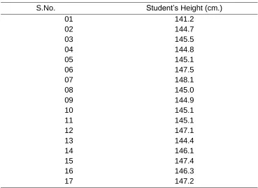
The application of the test is based on purely hypothetical data in Table-1

Table 1 Hypothetical Data

S.No. Student’s Height (cm.)

01 141.2

02 144.7

03 145.5

04 144.8

05 145.1

06 147.5

07 148.1

08 145.0

09 144.9

10 145.1

11 145.1

12 147.1

13 144.4

14 146.1

15 147.4

16 146.3

17 147.2

Mean= 145.6294

Standard Deviation (s) is = 1.626639

Range (w) of the data = 6.9

Null Hypothesis (H0): The sample data are not significantly different than a normal population.

Alternative Hypothesis (H1): The sample data are significantly different than a normal

population.

Q = w/s = 6.9/1.626639 = 4.24

In this case critical range at 5% level of significance and n=17 lower limit is 3.06 and upper limit

Licensed under Creative Common Page 6 Jarque–Bera test (Shapiro, 1980; Stuart et al., 1999)

This test is based on chi square means goodness of fit. Jarque -Bera test is based on skewness

(Sk) and kurtosis (Ku). The value of Jarque-Bera test (JB) is compared to the critical value of

Chi-Square (χ2_{) with 2 degree of freedom.}

Sk={∑ (yi – ӯ)3} / n . s3 ; i=1,2,…..,n

Ku = { ∑ (yi – ӯ)4} / n . s4 ; i=1,2,…..,n

Where y is the each observation is the standard deviation and n is the sample size.

JB= n[(Sk)2/6 + (Ku)2/24]

Application of the test is based on purely hypothetical data in Table-1.

Null Hypothesis(H0): Height is not significantly different than normal.

Alternative Hypothesis (H1): Height is significantly different than normal.

In this case critical value of Chi –Square is 5.991 at 2 degree of freedom.

Application on the same hypothetical data presented in the table.

N= 17 Mean (ӯ) = 145.6294

∑ (yi – ӯ) = 0.000 ; i=1,2,…..,17

∑ (yi – ӯ)2 = 42.3353 ; i=1,2,…..,17 ∑ (yi – ӯ)3 = -56.4694 ; i=1,2,…..,17 ∑ (yi – ӯ)4 = 459.3839 ; i=1,2,…..,17

Sk = { ∑ (yi – ӯ)3

} / n . s3 = -0.7718

Ku = { ∑ (yi – ӯ)4} / n . s4 = 0.8598

JB= n[ (Sk)2/6 + (Ku)2/24] =2.2112

In this case critical value of Chi –Square is 5.991 at 2 degree of freedom is greater than

calculated value of JB test. Therefore, H0 is accepted and conclude that height is not

significantly different than normal.

D'Agostino's or D Normality test

This is very powerful test based on D statistic. Statistic (D) is derived through sum of squared

deviates of data (SS) and sample size. First the data are arranged in ascending or descending

order (Stephens 1986).

D = T/√[(n3

x SS)]

T= ∑ [ i–{(n+1)/2}] yi

Application on the same hypothetical data presented.

Null Hypothesis(H0): Height is not significantly different than normal.

Alternative Hypothesis (H1): Height is significantly different than normal.

Licensed under Creative Common Page 7 Critical value of D= 0.2587, 0.2860

n= 17 Mean (ӯ) = 145.6294 (n+1)/2= 9

SS= ∑ (yi – ӯ)2

= 42.3353 ; i=1,2,…..,17

T=∑ (i-9)yi ; i=1,2,…..,17

T= (1-9)141.2+……….. +(17-9)148.1

T= 120.2

D = T/√[(n3 _{x SS)] = 120.2/ √[(17^3 x 42.3353)] = 0.2636}

Since 0.2587 < D=0.2636< 0.2860.

Therefore, H0 is accepted and conclude that the heights of the students are not significantly

different from normal.

Misc. Tests

Some other test for normality are defined as:

Kolmogorov–Smirnov test

Kolmogorov–Smirnov test statistic and its asymptotic distribution under the null hypothesis were

published by Kolmogorov (1933), while a table of the distribution was published by Smirnov

(1948). Recurrence relations for the distribution of the test statistic in finite samples are

available.

Under null hypothesis that the sample comes from the hypothesized distribution F(y),

√n Dn →sup│B F(t)│ if n → ∞

in distribution, where B(t) is the Brownian bridge.

If F is continuous then under the null hypothesis√n Dnconverges to the Kolmogorov distribution,

which does not depend on F. This result may also be known as the Kolmogorov theorem.

The goodness-of-fit test or the Kolmogorov–Smirnov test is constructed by using the critical values of the Kolmogorov distribution. The null hypothesis is rejected at level α if

√n Dn> Kα

WhereKα is found from

P(K ≤ Kα) = 1 - α

The asymptotic power of this test is 1.

Anderson–Darling Test

The Anderson–Darling test is a statistical test of whether a given sample of data is drawn from a

given probability distribution. In its basic form, the test assumes that there are no parameters to

be estimated in the distribution being tested, in which case the test and its set of critical values

Licensed under Creative Common Page 8 distributions is being tested, in which case the parameters of that family need to be estimated

and account must be taken of this in adjusting either the test-statistic or its critical values. When

applied to testing if a normal distribution adequately describes a set of data, it is one of the most

powerful statistical tools for detecting most departures from normality (D’Agostino et al., 1990;

Anscombe, et al. 1983).K-sample Anderson–Darling tests are available for testing whether

several collections of observations can be modeled as coming from a single population, where

the distribution function does not have to be specified.

In addition to its use as a test of fit for distributions, it can be used in parameter estimation as

the basis for a form of minimum distance estimation procedure.

Shapiro-Wilk test

The Shapiro–Wilk test is a test of normality in frequent statistics. It was published by Shapiro

and Wilk (1965).

The Shapiro–Wilk test utilizes the null hypothesis principle to check whether a sample y1, ...,yn

came from a normally distributed population. The test statistic is:

W = (∑ aiyi)2 / ∑(yi – ӯ)2 ; i= 1, 2, ………,n

where

yi(with parentheses enclosing the subscript index i) is the ithorder statistic, i.e., the ith-smallest

number in the sample

ӯ = [∑ yi]/n

the constants ai given by

yi (with parentheses enclosing the subscript index i) is the ithorder statistic, i.e., the ith-smallest

number in the sample, ӯis the sample mean and the constants ai are given by

(a1, a2, ………..,an) = [mTV-1]/(mt V-1V-1m)1/2

and m= (m1, m2, ………..,mn)T

Where, m1, m2, ………..,mn are the expected values of the order statistics of independent and

identically distributed random variables sampled from the standard normal distribution, and V is

the covariance matrix of those order statistics. The user may reject the null hypothesis if W is

below a predetermined value.

Omnibus K2 statistic

Statistics Z1 and Z2 can be combined to produce an omnibus test, able to detect deviations from

normality due to either skewness or kurtosis (D’Agostino, et al. 1990; Anscombe, 1983).

K2 = Z1(g1)2 + Z2(g2)2

If the null hypothesis of normality is true, then K2 is approximately χ2-distributed with 2 degrees

Licensed under Creative Common Page 9 Note that the statistics g1, g2 are not independent, only uncorrelated. Therefore their transforms

Z1, Z2 will be dependent (Shenton and Bowman, 1977).

DATA TRANSFORMATION

Data transformations are the application of a mathematical modification to the values of

variable. There are different variety of possible data transformations ranging from adding

constants to multiplying, squaring, converting to logarithmic scales, taking the square root of the

values and even applying trigonometric transformations. In other words data transformation is

the application of deterministic mathematical function to each point in a data set. Suppose each

data point Xi is replaced with the transformed value Yi = f(Xi) where f is a function.

Transformations are usually applied so that the observational data more closely meet the

assumptions of statistical procedure. Finally, transformed data improves interpretability, even if

formal statistical technique is to be used (Baker, 1934).

Concept and Meaning of Transformation Approach (Bartlett, 1947)

Y = α + β X (1)

It means that a unit increase in X is associated with an average of β units increase in Y.

log (Y)= α + β X (2)

Taking exponential both sides of equation (2)

Y= eα eβX

It means that a unit increase in X is associated with an average of 100β% increase in Y

Y= α + β log (X) (3)

It means that a 1% increase in X is associated with an average β/100 units increase in Y log(Y)= α + β log (X) (4)

Taking exponential both side of the equation (4)

Y = eα Xβ

It means that 1% increase in X is associated with a β% increase in Y

Transformations

The square root and logarithmic transformations are generally used for positive data. The

reciprocal or multiplicative inverse can be used for non- zero data. The power transformation is

a group of transformations with parameter λ (non negative value) that includes square root,

logarithmic and reciprocal transformation. It is possible to use statistical estimation procedure to

estimate the parameter λ in the power transformation. In the group of power transformation also

Licensed under Creative Common Page 10 would be best to analyze the data without transformation. In the regression analysis approach,

this technique is known as Box-Cox technique.

Square Root Transformation

Square root transformation is more common and popular data transformation. In this

transformation, the square root of every observation is taken. However, as one cannot take the

square root of a negative number, if there are negative values for a variable a constant must be

added to move the minimum value of the distribution above 0, preferably to 1.00. Another

important point is that numbers of 1.0 and above behave differently than numbers between 0.00

and 0.99. The square root of numbers above 1.0 always become smaller, 1.00 and 0.00 remain

constant, and numbers between 0.00 and 1.00 become larger. Thus, if apply a square root to a

continuous variable that contains values between 0 and 1 as well as above 1, treating some

numbers differently than others (Osborne, 2002).

Logarithmic Transformation

Logarithmic transformations are a class of transformations. In this transformation, logarithm is

the power a base number must be raised to in order to get the original number. Any given

number can be expressed as y to the x power in an infinite number of ways. It means that if

considering base 10, 1 is 100, 100 is 102, 16 is 101.2, and so on. Thus log10(100)=2 and

log10(16)=1.2 . Another common option is the natural logarithm, where the constant e (2.7183) is

the base. In this case the natural log 100 is 4.605. Logarithm of any negative number or number

less than 1 is unidentified, if a variable contains values less than 1.0 is constant must be added

to move the minimum value of the distribution, preferably to 1.00 (Osborne, 2002).

CONCLUSIONS

Research investigation is the part of a wider development with regard to finance, education,

public health, and agriculture, etc. that are indicators of better life of human beings. Modern

applied research based on better living management is quite complex, requiring multiple sets of

skills such as agricultural, medical, social, technological, mathematical, statistical etc. Suitable

statistical tools and research designs provide the unbiased estimates of the indicators,

conclusions, and their interpretations. The statistical tools are simple and applicable in various

fields and also some software’s are available for calculations of the statistical test. On the other

hand, assumptions and technicality behind the statistical tools and suitability of the tests are

also more important. In this context, normality is one of the most important aspects for statistical

analysis. Normality condition is essential especially for parametric test and regression analysis.

Licensed under Creative Common Page 11 statistical tests for normality are also useful for small sample sizes. A careful consideration of

normality and data transformation will hopefully result in more meaningful studies whose results

and interpretations are based on sound scientific principles.

REFERENCES

A1tman, D.G.& Bland, J. M. (1995). Statistics notes: the normal distribution, BMJ, 310(6975):298.

Anscombe, F.J. & Glynn, W. J. (1983).Distribution of the kurtosis statistic b2 for normal statistics, Biometrika, 70 (1): 227–234.

Baker, G. A. (1934). Transformation of non-normal frequency distributions into normal distributions. Annals of Mathematical statistics, 5, 113-123.

Bartlett, M. S. (1947). The use of transformation. Biometric Bulletin, 3, 39-52.

Casella, G& Berger, R. I. (2002). Statistical Inference, Second Edition.

Corder, G. W., Foreman, D. I. (2009).Nonparametric Statistics for Non-Statisticians: A Step-by-Step Approach. Wiley.

Cover, T. M. & Thomas, J. A. (2006).Elements of Information Theory, John Wiley and Sons.

D’Agostino, Ralph B., Albert Belanger, Ralph B. &D’Agostino, Jr. (1990).A suggestion for using powerful and informative tests of normality. The American Statistician, 44 (4): 316–321.

D’Agostino, Ralph B., Albert Belanger, Ralph B.& D’Agostino, Jr. (1990). A suggestion for using powerful and informative tests of normality.The American Statistician, 44(4): 316–321.

Driscoll, P., Lecky, F.& Crosby, M. (2000).An introduction to everyday statistics-1. Jr. Accid. Emerg. Medicine, 36(3):205-11.

Eadie, W.T., D. Drijard, F.E. James, M. Roos & B. Sadoulet (1971).Statistical Methods in Experimental Physics, Amsterdam: North-Holland.

Ghasemi, A. &Zahediasl, S. (2012). Normality test for statistical analysis: A guide for non- statistician. Int. Jr. of Endocrinology & Metabolism, 10(2), 486-489.

Kolmogorov A (1933). Sulla determinazioneempirica di unalegge di distribuzione.G. Ist. Ital. Attuari, 4: 83–91.

Osborne, J. (2002). Notes on the use of data transformations, Practical Assessment, Research and Evaluation, 8(6).

Oztuna, D., Elhan, A.H. & Tuccar, E. (2006).Investigation of four different normality test in terms of type 1 error rate and power under different distributions, Turkish Journal of Medical Sciences, 36(3): 171-6.

Royston, P. (1991).Estimating departure from normality. Stat. Medicine, 10(8):1283-93.

Shapiro, S. S. &Wilk, M. B. (1965).An analysis of variance test for normality (complete samples), Biometrika, 52 (3–4): 591–611.

Shapiro, S.S. (1980). How to test normality and other distributional assumptions. In: The ASQC basic references in quality control: statistical techniques, 3, 1–78.

Shenton, L.R. & Bowman, K.O. (1977).A bivariate model for the distribution of √b1 and b2. Journal of the American Statistical Association, 72 (357): 206–211.

Shorack, G.R. &Wellner, J.A. (1986).Empirical Processes with Applications to Statistics, Wiley.

Smirnov, N. (1948). Table for estimating the goodness of fit of empirical distributions. Annals of Mathematical Statistics, 19: 279–281.

Stephens, M. A. (1986). Tests Based on EDF Statistics, In D'Agostino, R.B. and Stephens, M.A. Goodness-of-Fit Techniques. New York: Marcel Dekker.