An Adaptive Controller using Radial Basis Function
Neural Network with Reinforcement Learning
Niusha Shafiabady
School of Electrical Engineering University of Nottingham
Malaysia Campus
M.A. Nima Vakilian
Planetary Science Institute Arizona
USA
Dino Isa
School of Electrical Engineering University of Nottingham
Malaysia Campus
ABSTRACT
A self-tuning PID control strategy using reinforcement learning is given to deal with conventional tracking control problems. Actor-Critic learning is used to tune PID parameters in an adaptive way to take advantage of the reinforcement learning properties. This policy is model-free and RBF neural network is used to approximate the parameters of PID controller. The critic part is designed to evaluate the actor part’s efficiency and compensate its disabilities producing TD error that is calculated by the temporal difference of the value function between successive states in the state transition. The inputs of RBF network are system error, as well as the first and the second order differences of error. Both PSO and gradient descent are used to train the network’s parameters and the controller has had a good performance being applied on the four plants.
Keywords
Reinforcement learning, Particle Swarm Optimization, Gradient Descent, Adaptive controller, Radial Basis Function, Fuzzy Neural Network
1.
INTRODUCTION
PID controllers are one of the most practical, reliable and typical controllers used for controlling variety of systems in many engineering fields. The controllers’ adaptive property is of great importance that is missing in conventional PID controllers, so the common design idea for adaptive PID controllers has received a wide attention in control activities. When a PID controller adapts itself to the changes in the plant and is model-free, it can obtain more satisfactory control effects. The conventional ways for designing PID controllers are dependent on the plant model that is not always available. Different adaptive PID controllers [5, 6] like fuzzy adaptive PID controllers [3], adaptive PID controllers based on neural networks [4] and evolutionary algorithms [2] have attracted a lot of attention in recent years. Needing to have the least knowledge of the controlled plant is one of the priorities of these kinds of controllers. Fuzzy adaptive PID controllers need to have some prior knowledge of the plant but the adaptive controller used here is model-free.
In this paper the reinforcement learning is used for controller design. This learning method unlike supervised learning of neural networks, adopts a ‘trial and error’ mechanism existing in human and animal learning [1]. This method emphasizes that an agent can obtain a goal from interactions with the environment. At first a reinforcement learning agent exploits the environment actively and then evaluates the exploitation results based on which the controller is modified. Actor-Critic learning is widely used in artificial intelligence, robot planning and control and optimization and scheduling fields.
Although there is no proof for these kinds of controllers’ stability, this interaction usually leads to a good controlling ability for the systems that can be controlled by an adaptive PID controller. In this paper the actor-critic part is implemented using RBF neural network and the PID controller’s parameters are updated using reinforcement learning placed in the error estimation of the used neural network.
This paper is organized as follows. In section 2 the adaptive network algorithmic implementation is explained. Section 3 presents the simulation results. Finally section 4 represents the conclusion.
2.
ADAPTIVE PID CONTROLLER
BASED ON REINFORCEMENT
LEARNING
2.1
Controller Architecture
The PID controller should be designed in a way that the error vector, including the error, the first-order and also the second order differences of error, would be minimized. The PID controller based on actor-critic learning illustrated in Fig. 1, is based on the design idea of the incremental PID controller described in Eq. (1).
)
(
)
(
)
(
)
1
(
)
(
)
(
)
(
)
1
(
)
(
)
(
)
1
(
)
(
)
1
(
)
(
2 3 2
1
t
e
k
t
e
k
t
e
k
t
u
t
x
k
t
x
k
t
x
k
t
u
t
x
t
K
t
u
t
u
t
u
t
u
D P
I
D P
I
(1)
Where () [ (), (), ()] [ (), (), 2 ()] 3
2
1 t x t x t et et et
x t
x and
)
1
(
)
(
)
(
),
(
)
(
)
(
t
y
t
y
t
e
t
e
t
e
t
e
desired and also)
2
(
)
1
(
2
)
(
)
(
2
e
t
e
t
e
t
e
t
. Here is a vector of PID parameters.In Fig. 1. y(t) and Ref on the top show the actual output and the reference input respectively. The error e(t) is used as the system state vector input that is x(t) and is needed by the actor-critic part. Actor-critic learning architecture has three different parts, including a critic, an actor and a stochastic action modifier called SAM. The actor suggests the mapping from the current system state vector to the recommended PID
parameters K(t)[kI(t),kP(t),kD(t)] that are not the actual
PID parameters and won’t be applied to the controller directly. The critic is planned to generate the signal V(t).The SAM is used to create and finalize the actual PID parameters
K(t) according to recommended PID parameters K(t) proposed by the actor and the estimated signal V(t) from the critic.
The critic part’s inputs are the system state vector and an external reinforcement signal that is the reward r(t) from the environment and produces a TD error that is the internal
reinforcement signal TD(t)and an estimated value function
V(t). TD(t) that is provided for the actor and the critic plays an important role in updating the parameters of the actor and the critic. V(t) is sent to the SAM and for modifying the output of the actor. The control performance, the system error and also the change of error rate have to be considered to produce the reward r(t). Finally r(t) will be defined as:
)
(
)
(
)
(
t
r
t
r
t
r
e
e
(2)
otherwise
t
e
t
e
t
r
otherwise
t
e
t
r
e e
5
.
0
)
1
(
)
(
0
)
(
5
.
0
)
(
0
)
(
(3)
Where α and β are weighting coefficients and ε is the estimated error band.
2.2
RBF Neural Network
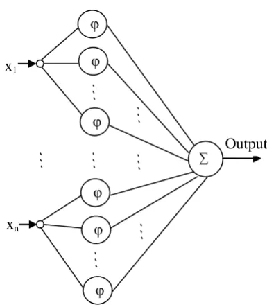
The structure of RBF neural network is shown in Fig. 2. The output is calculated as mentioned in Eq. (4).
n n
w
w
w
out
1*
1
2*
2
...
*
(4)Where
exp ( 2 )2
i i i i
m x
and
m
iand
i are thecenters and the standard deviations. Since RBF neural network looks like a fuzzy system without an inference engine we are going to call the first layer and the output layer,
antecedent and conclusion parts respectively [8]. So
m
iandi
are considered to be the antecedent part's parameters whereas the conclusion part’s parameters arew
i as mentioned in Eq. (4). This type of neural network is proposed to be used for its good generalization ability.Fig 2: The structure of RBF neural network
2.3
Particle Swarm Optimization
PSO is an evolutionary optimization algorithm that has been widely used for optimization problems because of its efficient outcome in recent years. It consists of some particles that each has a velocity and a position. The particles move on until a desired goal is achieved by the particle with the best experience called global best. Each particle’s best experience happens in a particle called personal best. It is formulated as Eq. (5).
max 1
_ 2
_ 1
1
1
1
5
.
0
1
)
(
)
(
t
t
w
V
X
X
X
X
c
rand
X
X
c
rand
wV
V
i i i
Term Social
i Bset iGlobal
Term Cognitive
i Best iPersonal i
i
(5)
Where c1 and c2 are positive constants that show the emphasize put on the cognitive or social terms, and rand is a random number. For PSO to converge c1c24 should be
supported. The inertia weight is named w here. The variables
1
c
andc
2 are used to keep the balance related to the abilities of local and global search that is important in the algorithm’ssuccess. In this study c1c21that is found by ‘try and
error’.
t
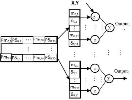
max is the maximum number of iterations that is assumed to be 50 by ‘try and error’ and t is the current iteration.The shortcoming of this technique is said to be its long execution time. This can be solved by reducing the number of the particles that hardly shows any effect in the given results and speeds up the algorithm. In this paper, PSO is used to find the antecedent and the conclusion parts’ parameters of the RBF neural network. For training the antecedent part’s parameters, as there is no fitness function to show the efficiency of the chosen particles, so to solve this issue some
x
1x
n∑
φ
φ
φ
φ
φ
φ
parallel networks have to run for the global best to be chosen. This is shown in Fig. 3. The network shown in the figure 3 has eleven neurons and PSO algorithm has been used with 30 particles applied to 10 parallel networks as shown in Fig 3.
Fig 3: The structure of parallel RBF neural networks using PSO to find the antecedent part’s parameters [8]
2.4
Actor-Critic Learning Based on RBF
Neural Network
The RBF neural network used here accepts the error vector
that is
[
(
),
(
),
(
)]
2e
t
t
e
t
e
as its input and produces twoseries of outputs. The first group of outputs are the
recommended PID parameters
)]
(
),
(
),
(
[
)
(
t
k
t
k
t
k
t
K
I
P
D
and the second output that is a single one is the estimated value function V(t) known as critic value, as shown in Fig 4.
Fig 4: Actor-Critic learning based on RBF neural network [5]
A Gaussian noise
n
kthat is zero-mean with the magnitude)
(
t
v
, that depends on V(t), is added to the recommendedPID parameters
K
(
t
)
as mentioned in Eq. (6).))
(
,
0
(
)
(
)
(
t
K
t
n
t
K
k
v (6)Where
))
(
2
exp(
1
1
)
(
t
V
t
v
This means that if V(t) is small
n
kis large and vice versa.The actor-critic learning indicates two different roles. The actor learns the policy function and the critic learns the value function using the TD method [6]. The TD error is calculated as shown in Eq. (7).
)
(
)
1
(
)
(
)
(
t
r
t
V
t
V
t
TD
(7)Where r(t) is the external reinforcement reward signal and
1
0
denotes the factor that is used to determine theproportion of the delay to the future rewards. The TD error shows how much the actual action is approved. Therefore the performance function of the system learning can be defined as follows.
2 2 1 ) (t TD
E
(8)Based on the mentioned performance, the weights of the network are trained using PSO and gradient descent methods. According to chain rule, the weights’ updating algorithm is mentioned in Eq. (9).
) ( ) ( ) ( ) 1 ( ) ( ) ( ) ( ) ( ) ( ) ( ) 1 ( t t t v t v t t t K t K t t w t w j TD C j j j v m m TD A mj mj
(9)Where m=1, 2, 3 that denotes the number of the inputs and j defines the number of the hidden unit’s neurons that are
considered 11 in our study by ‘try and error’ method.
AandC
are learning rates.2.5
Controller Design Steps
The controller is designed taking the following steps.
At first the parameters of the controller are initialized.
For t=1: maximum repititions
o Compute the error by deducting y(t) from the desired output
o Receive the reward r(t)
o Compute the Actor output and the Critic Value
o Calculate the PID gains and compute u(t) accordingly.
o Apply the control input to the system and compute the output and define the new reward for the next iteration, together with Actor output and the Critic function for the next step.
o Find their related error and update the Actor and Critic's weights and update the RBF neural network's Gaussian parameters accordingly.
The numbers of the repetitions in the loop are computed by the sampling time and the overall runtime of the program in seconds. ϕ ϕ ϕ . . . e(t) ∆e(t)
∆2e(t) Actor
for PID Gains Critic ∑ ∑ φ φ φ φ
X
,
Y
m
0 , 1m
0 , 1 1σ
0 , 1σ
0 , 1P
σ
9 , 1P
m
9 , 1P
σ
9 , 3 0P
m
9 , 3 0P
σ
0 , 1P
m
0 , 1P
σ
0 , 3 0P
m
0 , 3 0m
9 , 1m
9 , 1 1σ
9 , 1σ
9 , 1 Output0 Output9 X,Y m0,1 δ0,1Pm9,1 Pδ9,1
Pδ0,1
Pm0,1 Pm0,30 Pδ0,30
2.6
Simulation Results
The controller has been simulated on four plants using Matlab. For all the plants, the desired trajectory is assumed to be step and sine function. The first system’s equation is as follows [5].
)
8
.
0
1
(
2
.
1
)
2
(
)
1
(
)
1
(
1
)
1
(
)
(
) ( 01 . 0 2
max
t t
e
a
t
u
t
u
t
y
t
ay
t
y
(10)
Here a is considered to examine the robustness of the system.
For all the simulations the parameters
=0.6,
=0.4,
=0.01,
=0.98,
A=0.013, C
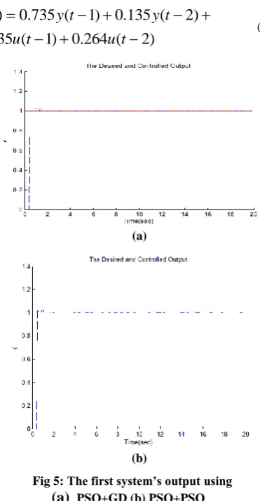
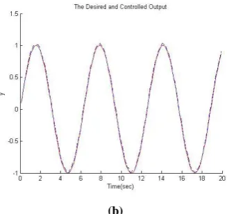
=0.01 and Ts=0.001s. Fig. 5.a shows the first system’s result, tracking step response, using gradient descent for training the conclusion part’s parameters and PSO to achieve the antecedent part’s parameters. Fig. 5.b shows the result using PSO for training both parts’ parameters. Fig. 6 shows the same results tracking sine signal. In all the given results the dotted line shows the system’s output.The second plant’s equation is as follows in discrete form [7].
)
2
(
264
.
0
)
1
(
135
.
0
)
2
(
135
.
0
)
1
(
735
.
0
)
(
t
u
t
u
t
y
t
y
t
y
(11)
(a)
(b)
Fig 5: The first system’s output using
(a)
PSO+GD (b) PSO+PSOFig. 7.a shows the second system’s result, tracking step signal, using gradient descent for training the conclusion part’s parameters and PSO to achieve the antecedent part’s parameters. Fig. 8.b shows the result using PSO for training
both parts’ parameters and Fig. 8 shows the same result tracking sine signal.
(a)
(b)
Fig 6: The first system’s output using
(a) PSO+GD (b) PSO+PSO
(a)
(b)
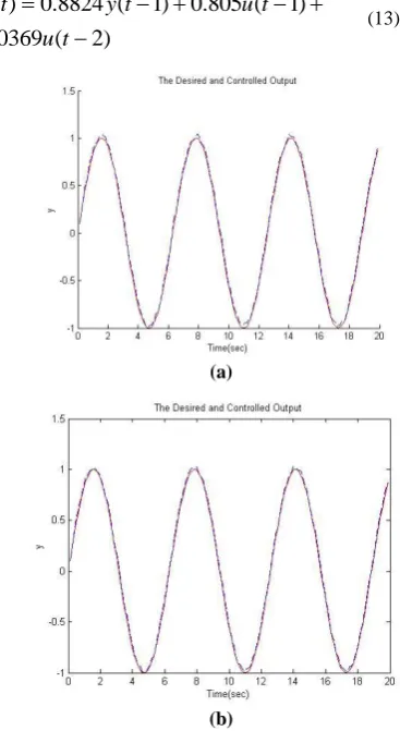
The third plant is the stirred tank process [7] with the equation mentioned below.
143
)
(
6 . 9
s
e
s
G
s
(12)
That is will be displayed as mentioned below in discrete form.
)
2
(
0369
.
0
)
1
(
805
.
0
)
1
(
8824
.
0
)
(
t
u
t
u
t
y
t
y
(13)
(a)
(b)
Fig 8: The second system’s output using
(a) PSO+GD (b) PSO+PSO
The simulation results of this system is given in Fig. 9 to track step response and Fig. 10 to track sine signal, where the result that gradient descent is used for training the conclusion part’s parameters and PSO to achieve the antecedent part’s parameters, are given in Fig. 9.a. and Fig. 10.a. and the result after using PSO for training both parts’ parameters, are given in Fig. 9.b. and Fig. 10.b.
(a)
(b)
Fig 9: The first system’s output using
(a) PSO+GD (b) PSO+PSO
Finally the fourth system denotes a system with the following equation [7].
)
1
)(
1
2
.
0
(
2
)
(
2 . 0
s
s
e
s
G
s
(14)
Where the equation in discrete form is as mentioned in Eq. (15).
)
4
(
0337
.
0
)
3
(
0412
.
0
)
2
(
5488
.
0
)
1
(
5114
.
1
)
(
t
u
t
u
t
y
t
y
t
y
(15)
(a)
(b)
Fig 10: The third system’s output using
Finally the simulation results of the fourth system are given in Fig.11 and Fig.12 tracking step and sine signals respectively.
(a)
(b)
Fig 11: The first system’s output using
(a) PSO+GD (b) PSO+PSO
The results of all four systems show that both ways for parameter assignment for the controllers have been successfully efficient but PSO has been able to give better performance to the systems to follow the trajectory better. By decreasing the number of the particles used for PSO, the fast training speed could be maintained.
(a)
(b)
Fig 12: The third system’s output using
(a) PSO+GD (b) PSO+PSO
3.
CONCLUSION
Simulation results indicate that the adaptive PID controller can perform the tracking control task efficiently. Based on reinforcement learning ability it can adapt itself well and is also model-free. Both parameter training methods have performed well, but having compared the results, PSO has been able to achieve better results. This is because of the ability of PSO in good exploitation and the proper exploration of the search space that has enforced the controller to be tuned properly and at the same time the reinforcement learning itself is a good control strategy especially when used for the adaptive systems.
This can be proposed as a good tracking control method for the control tasks that accuracy is of great importance for them.
4.
REFERENCES
[1] Cheng Y H, Yi J Q, Zhao D B. Application of Actor-Critic Learning to Adaptive State Space Construction. Proceeding of the Third International Conference on Machine Learning and Cybernetics. Shanghai, Institute of Electrical and Electronics Engineers Inc. Press, 2004, 26-29.
[2] Kondo T, Ito K., A Reinforcement Learning with Evolutionary State Recruitment Strategy for Autonomous Mobile Robots Control, Robotics and Autonomous Systems, 2004,46(2), 111-124.
[3] Zhou KT, Zhen L X, Optimal Design of PID Parameters Using Evolutionary Algorithms, Journal of Huaquiao University (Natural Science), 2010, 26(1), 85-88.
[4] Wang X S, Cheng Y H, Sun W Q, Learning Based on Self Organizing Fuzzy Radial Basis Function Network, Lecture Notes in Computer Science, 2006, 3971, 607-615.
[5] Wang Xue-song, Cheng Yu-hu, Sun Wei, A Proposal of Adaptive PID controller, China Univ Mining & Technology, 2007, 17(1), 40-44.
[6] Barto A G, Sutton R S, Anderson C W, Neuronlike Adaptive Elements that can Solve Difficult Learning Control Problems, IEEE transactions on Systems, Man and Cybernetics, 13(5), 834-846.
[8] Niusha Shafiabady, M. Teshnehlab, M. Aliyari, A Comparison of PSO and Backpropagation Combined with LS and RLS in Identification Using Fuzzy Neural Networks, 2006 IEEE International Conference on Industrial Technology.
[9] You-tong, F., Cheng-zhi, F., Single neuron network PI control of high reliability linear induction motor for Maglev. Journal of Zhejiang University SCIENCE A, 2010, 8(3):408-411.
[10]Gwo-Ruey Yu and Lun-Wei Huang , “Design of LMI-Based Fuzzy Controller for Two-link Robot Arm using Genetic Algorithms,” Proceedings of 2008 CACS International Automatic Control Conference National Cheng Kung University, Tainan, Taiwan, Nov, 21-23, 2008.
[11]A. Oonsivilai and P. Pao-La-Or, “Application of adaptive tabu search for optimum PID controller tuning AVR system,” WSEAS Transactions on Power Systems, vol. 3, no. 6, pp. 495–506, 2008.
[12]C. Cao, X. Guo, and Y. Liu, “Research on ant colony neural network PID controller and application,” inProceedings of the 8th ACIS International Conference on Software Engineering, Artificial Intelligence, Networking, and Parallel/Distributed Computing (SNPD '07), pp. 253–258, 2007.
[13]A. Bagis, “Determination of the PID controller parameters by modified genetic algorithm for improved performance,” Journal of Information Science and Engineering, vol. 23, no. 5, pp. 1469–1480, 2007.
[14]K. Sansal, Y. ildiz, Biao Huang, J. Fraser Forbes, Dynamics and variance control of hot mill loopers, Control Engineering Practice, vol. 12, no. 16, 89-100,
2008.
[15]Bin-hu Yang, Wei-dong Yang, Lian-gui Chen, Lei Qu, Dynamic optimization of feed forward automatic gauge control based on extend Kalam Filter, International Journal of Iron and Steel, vol. 15, no. 2, 39-42, 2008.
[16]S. I. Han, K. S. Lee, M. G. Park, and J. M. Lee, “Robust adaptive deadzone and friction compensation of robot manipulator using RWCMAC network,” Journal of Mechanical Science and Technology, vol. 25, no. 6, pp. 1583–1594, 2011.
[17]M. M. Fateh and S. Khorashadizadeh, “Robust control of electrically driven robots by adaptive fuzzy estimation of uncertainty,” Nonlinear Dynamics, vol. 69, no. 3, pp. 1465–1477, 2012.
[18]Hou, G. l., Zhang, J. F., Liu, J. J., and Zhang, J. H., “Multiple-Model Predictive Control Based on Fuzzy Adaptive Weights and Its Application to Main-Steam Temperature in Power Plant,” IEEE Conference on Industrial Electronics and Applications , pp. 668–673, 2010.
[19]Du, H. P., and Zhang, N., “Static Output Feedback Control for Electrohydraulic Active Suspensions via T–S Fuzzy Model Approach,” ASME J. Dyn. Syst., Meas., Control, 131 (5), p. 051004, 2009.
[20]Daogang Peng, Hao Zhang, Hui Li, and Fei Xia, "Research of Networked Control System Based on Fuzzy Adaptive PID Controller," Journal of Advances in Computer Networks vol. 2, no. 1, pp. 44-47, 2014.
![Fig 1: Self-adaptive PID controller based on reinforcement learning [1]](https://thumb-us.123doks.com/thumbv2/123dok_us/1258595.1631451/1.595.315.542.538.766/fig-self-adaptive-pid-controller-based-reinforcement-learning.webp)