Investigation of Selected Versions of Fourth Order Runge-Kutta Algorithms as Simulation Tools for Harmonically Excited Nonlinear Pendulum

(1)

_____________________________________________________________________________________________________

14(2): 1-12, 2018; Article no.ACRI.41110

ISSN: 2454-7077

Investigation of Selected Versions of Fourth Order

Runge-Kutta Algorithms as Simulation Tools for

Harmonically Excited Nonlinear Pendulum

Salau, T. A. Ogunniyi

1*

and Sedik Faruk

1

Department of Mechanical Engineering, University of Ibadan, Ibadan, Nigeria.

Authors’ contributions

This study was carried out in collaboration between both authors STAO and SF. Author STAO designed the study and wrote the protocol. Author SF managed the literature searches, wrote the FORTRAN code used and the first draft of the manuscript. Both authors managed the analysis of the study and read and approved the final manuscript.

Article Information

DOI: 10.9734/ACRI/2018/41110

Editor(s):

(1) Sanjeev Kumar, Professor, Department of Physics, Medical Physics Research Laboratory, D. A. V College, U.P, India.

Reviewers:

(1)Liangqiang Zhou, Nanjing University of Aeronautics and Astronautics, China. (2)Aliyu Bhar Kisabo, Nigeria. (3)Chaouchi Belkacem, Khemis Miliana University, Algeria. Complete Peer review History: http://www.sciencedomain.org/review-history/24742

Received 15th March 2018 Accepted 19th May 2018 Published 23rd May 2018

ABSTRACT

This study employed fifty-five selected versions of the Runge-Kutta (RK) fourth order schemes tagged (RKV_1, RKV_2, …, RKV_55), inclusive is the classical fourth order scheme RKV_55 to simulate the dynamics of harmonically excited nonlinear pendulum using adaptive time step technique over a range of drive parameters, initial conditions and excitation frequencies. A FORTRAN program was developed to carry out the simulation and validated by comparing Poincare section obtained with literature standard. The Poincare sections generated compares favourably with those published in literature, thus validate the algorithm. Furthermore, the study results show that number of steps each Runge-Kutta version used to complete the specified simulation periods of the nonlinear pendulum differs significantly. Ranking the versions by the number of steps indicated that RKV_55 is not the fastest version as other versions such as RKV_2, RKV_8, RKV_9, RKV_10, and RKV_51 outperformed it. In addition, the performance of these versions are not significantly affected by the change in initial condition but are greatly affected by the change in angular drive frequency.

(2)

Ogunniyi and Faruk; ACRI, 14(2): 1-12, 2018; Article no.ACRI.41110

Keywords: Harmonically excited; nonlinear pendulum; Runge-Kutta and variable time step.

1. INTRODUCTION

[1] defined dynamical system as any physical or abstract entity whose form at any given time can be defined by some set of numbers, called system variables, and whose configuration at a later time is uniquely determined by its present and past configurations through a set of rules for the transformation of the system variables.

Several engineering and science problems are usually modelled mathematically to form differential equations, such ordinary differential equations and partial differential equations [2]. Once the governing equation has been formulated analysis can proceed.

Analytical or exact methods were used to derive solutions for some of these problems. Useful insight into the behaviour of some systems were excellently provided, by these solutions. However, the class of problems that their analytical or exact solution can be derived are limited. Therefore, analytical solutions have restrained practical value since most engineering posed problems are nonlinear and involve complex shapes and process [3].

When engineering posed problems, becomes difficult to solve directly, transformation of the original system to an approximated one is usually done, and analysis is carried out due to the solution provided by the approximated system. However, because of the existence of some missing information in the approximation, one cannot say that the solution of the approximated system reflects the solution of the original system [4]. In most cases, numerical methods are broadly used for solving these mathematical problems developed in science and engineering where it is hard or yet impossible to obtain exact solutions because they give more accurate results and realistic error information [2].

Runge-Kutta ( RK) m e t h o d s a r e c o m m o n l y e m p l o y e d t o numerically solve IVPs (Initial Value Problems), because, they are well known for their speed and accuracy. Around the 1900, German Mathematicians C. Runge and M W. Kutta formulated the Runge-Kutta (RK) methods, and ever since it has become a crucial family of implicit and explicit iterative methods needed to estimate the solutions of ordinary differential equations. These methods solve higher order

derivative with high accuracy, even though they require less computation [5]. Fourth order RK methods are the most popularly used in solving most initial value problems. Similar to the second order methods, there are infinite versions of the fourth order method. The most commonly used fourth-order Runge-Kutta method is the classical fourth-order Runge-Kutta method [3].

[2] carried out a comparative study on numerical solutions of initial value problems for ordinary differential equations using Euler and Runge-Kutta method. The approximated solution of the solved differential equation and the maximum error obtainable was calculated for different step size 0.1, 0.05, 0.025 and 0.0125. The results indicated that the solution obtained numerically by the two proposed methods compares favourably with the exact solutions. Also, to increase the accuracy of the approximated solution for both methods a smaller step size should be used. He concluded that the Runge-Kutta method is more accurate and also the approximate solution converged faster to the exact solution when compared to the Euler method.

[6] in his work presents a numerical method for solving transient analysis in vibration analysis. The dynamic model of a combat vehicle was utilized, while the numerical simulation was conducted using Runge-Kutta fourth order method. The focus of the work was the discussion of the accuracy of numerical methods used to predict the value of deviation that occurs during the process of single shooting. The simulation results were observed to be unstable when the numerical approach of 0.01s time step was used, contrary to a time step of 0.001s that produced stable results. The study, therefore, confirmed the sensitivity of Runge-Kutta numerical method to time step selection.

(3)

q

constant time step integration of steady displacements and velocities for the Duffing’s equation so as to produce phase plots and Poincare sections. The Poincare sections generated by these versions from several agreeing driven parameters combination, compared favourably with those from literatures. The results also show some noticeable deviation, which was due to the adoption of lower order Runge-Kutta method. Finally, they were able to recheck and confirm the complicated and wide-ranging nature of the solutions to the Duffing’s equation.

An effective ordinary differential equation (ODE) integrator ought to maintain some adaptive power to direct or determine its own advancement, by making necessary changes in its step size. The main purpose of this adaptive step size control is to accomplish some preset accuracy in the solution with the least possible computational effort [8]. When the terrain is unstable and unpredictable many small steps are required, while few great strides should be used to speed through smooth terrains. The resulting gains in efficiency are not mere tens of percent’s or factors of two they can sometimes be factors of ten, a hundred, or more [8].

In designing an adaptive step size control scheme the most universal way lies in calculating the ‘local error’ at each step of the algorithm, that is the error made in computing the approximated solution at a given grid point assuming that the data from the previous grid point was exact [9]. The step size is then computed for every grid point, ensuring that the local error is lower than the predefined value called the tolerance. The value of the tolerance is set depending on the need for accurate results, for example to 10−q with q ranging from 3 to 9 [9].

[10] carried out a comparative analysis of time steps distribution in Runge-Kutta algorithms, this study utilizes combination of phase plots, time steps distribution and adaptive time steps Runge-Kutta fourth and fifth order algorithms to investigate a harmonically excited Duffing oscillator. The study objective was to visually compare the performance of fourth and fifth order Runge-Kutta as tools for seeking the chaotic solutions of a harmonically excited Duffing oscillator. The results show that, though fifth order algorithms favours higher time steps and as such faster to execute than fourth order for all studied cases, but at the expense of reliability of the computed results. This also contributes to

the fact that Runge-Kutta fourth scheme has been preferred and considered reliable than other schemes. In the aspect of time step selection, they set the tolerance (εt) of their solution at 10-6 for all the steps in the computation, while the local error(ε) compares the predicted results taking two half-steps with taking a full step for one of the module investigated.

From existing literatures, it is established that though the harmonically excited nonlinear pendulum has been studied in details using various Runge-Kutta schemes across different parameter space, there still exists a need to study the equation across other parameters using several versions of one of these methods. Therefore, this study seeks a solution reliable in speed to this system, using several versions of fourth order Runge-Kutta schemes.

2. METHODOLOGY

2.1 Harmonically Excited Nonlinear

Pendulum

This research is strictly based on the numerical simulation of the normalized governing equation of harmonically excited nonlinear pendulum given by equation (1) [11].

1

sin( ) gcos( Dt)

q

     (1)

In other to simulate equation (1) with any of fourth order Runge-Kutta schemes demands its transformation to a pair of first order differential equation (2) and (3) under the assumption that (θ_{1 = angular displacement}θ_{2 = angular}

velocity).

(2)

, , , , , (3)

The differential equation contains three changeable parameters which are: the driving force amplitude (g), the damping or quality parameter (q) and the angular drive frequency (ω_D)

2.2 The Fourth Order Runge-Kutta

For an arbitrary first order differential equation

(4)

Runge-Kutta predictive scheme is given by

equation (4).

(4)

Where h is the step size, the b’s are constant and the k’s are:

, (5)

, (6)

, (7)

,

(8)

The coefficients of equations (4) to (8) are defined as in table 1 in accordance with explanations provided by [12].

2.3 Versions of Fourth Order Runge-Kutta Adopted for This Study

Assuming that Table 1 by contents satisfies the fourth order conditions, then the values of these coefficients can be calculated from the general equations as explained by [12].

Table 1. Butcher’s tableau for general fourth order scheme

Using equations (2) and (3) above, the following transformations were made, so as to incorporate the governing equation of the harmonically excited nonlinear pendulum to the general fourth order Runge-Kutta method [13].

These quantities are then used in the following recurrence formula:

(9)

(10)

(11)

The coefficients of equations (9) to (11) are defined as in table 1 in accordance with explanations provided by [12].

2.4 Validation Cases

The under-listed parameters were used to test run the FORTRAN subroutines written for this study. The Poincare sections obtained for test cases were used to compare the published ones.

2.4.1 Test Case – I

, , ≡ 2, 1.5, , initial conditions (0, 0),

transient and steady simulation (50, 10000), number of simulation within a period (500).

2.4.2 Test Case – II

, , ≡ 4, 1.5, , initial conditions (0, 0),

transient and steady simulation (50, 10000), number of simulation within a period (500).

2.5 Time Step Selection

[3] argued that, there are limitations to the solution of the ordinary differential equation of some dynamical systems that demonstrate a sharp change when they are evaluated using constant time step size. To achieve the objective of this work, the step doubling adaptive time step technique was used. Equations (12) and (13) below were used to increase and decrease the time step (h) respectively. The tolerance (ε_t) was

set at 10-6 for all computation steps,

while the local truncation error (ε) was

calculated by comparing the predicted results taking two half-steps with taking a full step. Equation (12) is used if ε < ε_tand equation (13) is used if ε > ε_t.

/ (12)

/ (13)

From equations (12) and (13) above α is the step size control factor, which takes its value within the range (0 < α < 1). In this study, one

hundred and one (101) values of α which

(5)

Table 2. Transformation equations, for calculating the displacement and velocity of a

dynamical system

t , , , , ,

, ,

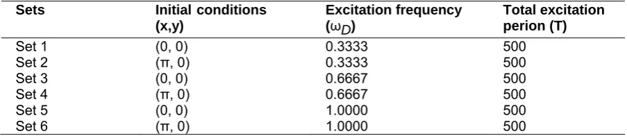
Table 3. Summary of investigated points on the study parameter plane

Sets Initial conditions

(x,y)

Excitation frequency (ω_D)

Total excitation perion (T) Set 1

Set 2 Set 3 Set 4 Set 5 Set 6

(0, 0) (π, 0) (0, 0) (π, 0) (0, 0) (π, 0)

0.3333 0.3333 0.6667 0.6667 1.0000 1.0000

500 500 500 500 500 500

To achieve this, a quick simulation was done using (RKV_2, RKV_8, RKV_9, RKV_10, RKV_51, and RKV_55) at (0, 0) initial condition. The simulation was done to a simulation time length of five hundred excitation periods and the total time steps were taken by each version for respective values of α collated and divided by their equivalent constant time steps to obtain the time step ratio.

2.6 Parameter Details of Studied Cases

A point on the parameter plane is defined as a case. 101 × 101 cases were investigated at three

different excitation frequencies

ω , 1.0 alongside uniform step

increment of damping coefficient ( 2.0≤q≤4.0 )

and forcing amplitude ( 0.9≤g≤1.5 ) over large number of excitation period at the equilibrium positions (0,0) and (π,0) as initial conditions for displacement and velocity respectively. The starting simulation time step for excitation

period . The simulations were performed

for 500-excitation periods, comprising 50-periods of unsteady and 450-periods of steady solutions. All integrations were carried out using the 55-selected versions of the popular Runge-Kutta fourth order using the adaptive time step integration suitably coded in FORTRAN-95.

From all the investigated points in the parameter plane, the versions were ranked from 1st to 55th position. The summary of the results considers only the versions in the first position at each point.

3. RESULTS AND DISCUSSION

Fig. 1 and Fig. 2 are typical Poincare sections for each validation case, which compares favourably with published Poincare sections in literature, thus validates the algorithm as shown by [11].

Fig. 3 shows that, as the value of increases, the time steps taken by each version to complete the simulation length reduces drastically making their time step ratio asymptotically approaching 10%, as approaches unity. Since the increase in the value of reduces the time step ratio for all versions, it is therefore safe and time saving to select the value of as close as possible to 1.0. As a result, (α = 0.95) was used for this study.

RKV_2, RKV_8, RKV_9, RKV_10 and RKV_51 dominated the remaining fifty versions including the classical Runge-Kutta fourth order in Set 1 to Set 4, while in Set 5 and Set 6 only three versions dominated the rest versions. Performance of the versions is not significantly affected by change in initial conditions, but are significantly affected by changes in angular drive frequencies.

(6)

Fig. 1. Poincare section for Validation Case-I

Fig. 2. Poincare section for Validation Case-II

(7)

Table 4. Coefficients for the classical and the top six versions from all selected versions of

fourth order Runge-Kutta schemes used

Coefficient Selected Versions Fourth order Runge-Kutta Scheme

RKV_2 RKV_8 RKV_9 RKV_10 RKV_51 RKV_55

c2 c3 c4 a21 a31 a32 a41 a42 a43 b1 b2 b3 b4 0.2551 0.7449 1.0000 0.2551 -0.7151 1.4600 4.2825 -5.1027 1.8203 0.0615 0.4385 0.4385 0.0615 0.1386 0.8614 1.0000 0.1386 -2.2461 3.1075 -6.4297 7.9183 -0.4886 -0.1980 0.6980 0.6980 -0.1980 0.1493 0.8507 1.0000 0.1493 -1.9983 2.8490 -6.7706 8.3981 -0.6275 -0.1561 0.6561 0.6561 -0.1561 0.2575 0.7425 1.0000 0.2575 -0.6992 1.4417 4.0018 -4.7515 1.7498 0.0641 0.4359 0.4359 0.0641 0.3333 0.6667 1.0000 0.3333 -0.3333 1.0000 1.0000 -1.0000 1.0000 0.1250 0.3750 0.3750 0.1250 0.5000 0.5000 1.0000 0.5000 0.0000 0.5000 0.0000 0.0000 1.0000 0.1667 0.3333 0.3333 0.1667

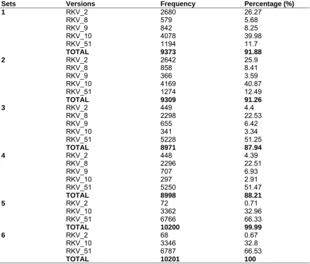
Table 5. Performance (first position) of top five versions across all Sets

Sets Versions Frequency Percentage (%)

(8)

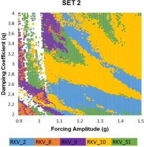
Fig. 4

Fig. 5

4. Regional d

5. Regional d

dominance o

of each vers p

Ogunniyi an

sion of the t plane in Set

nd Faruk; ACRI,

top five vers 1

top five vers 2

14(2): 1-12, 20

sions on the

018; Article no.A

e study para

ACRI.41110

ameter

(9)

Fig. 6

Fig. 7

6. Regional d

7. Regional d

dominance o

of each vers p

sion of the t plane in Set

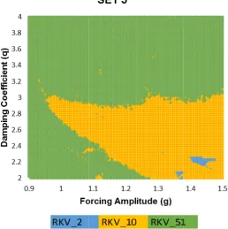
top five vers 3

top five vers 4

sions on the

e study para

ameter

(10)

Fig. 8.

Fig. 9.

Table 5 in the t

Regional d

shows the p top five ran

ominance o

performance nking positio

of each vers p

e of each ve on from the

Ogunniyi an

ion of the to plane in Set

rsion e RK versvers

nd Faruk; ACRI,

op three ver 5

op three ver 6

sions adopte sions varied

14(2): 1-12, 20

rsions on th

ed in this stu across the

018; Article no.A

he study par

udy. Perform simulated s

ACRI.41110

rameter

(11)

set in which the versions performed best are as

follows: RKV_2 set 1, RKV_8 set 3, RKV_9 set 2, RKV_10 set 2 and RKV_51 set 6 covering 2680 (26.27%), 2298 (22.53%), 858 (8.41%), 4169 (40.87%) and 6787 (66.53%) points respectively, from all the 10201 simulation points. Also the set in which the versions performed poorly are as follows: RKV_2 set 6, RKV_8 set 6, RKV_9 set 5 and set 6, RKV_10 set 4 and RKV_51 set 1 covering 68 (0.67%), 0 (00.00%), 0 (00.00%), 297 (2.91%) and 1194 (11.7%) points respectively, from all the 10201 simulation points.

In Figs. 4 to 9, each dot on the parameter plane gives the coordinate (q, g) in which a particular version in the top five versions took the first position, and also provide clearer picture of the region in the plane where a particular version dominates. It is observed that the versions behaviour is not truly affected by change in the initial conditions, but are greatly affected by change in angular drive frequency.

4. CONCLUSIONS

This research has developed an algorithm that can simulate the dynamics of harmonically excited nonlinear pendulum; using several selected versions of fourth order Runge-Kutta schemes with the step doubling adaptive time step technique, one of which is the classical fourth-order Runge-Kutta. The Poincare sections obtained compares favourably with those found in literature and thus validates algorithm developed. Five out of the fifty-five versions studied exhibited domination over the remaining versions including the classical Runge-Kutta fourth order in the first four sets while only three versions dominated in the last two sets investigated. Thus there are some versions of fourth order Runge-Kutta schemes that are faster than the classical fourth order scheme when the adaptive step size control with the step doubling method is employed. The versions performance is not significantly affected by change in initial conditions, but are significantly affected by changes in angular drive frequencies. While recommending all the top performing versions from this study preferentially as dynamics systems simulating tools further investigations with the same objective should be carried out on other versions not yet investigated.

COMPETING INTERESTS

Authors have declared that no competing interests exist.

REFERENCES

1. Socolar JES. Nonlinear dynamical systems. Deisboeck T, Kresh J, Eds. Physics Department, Duke University, Durham, North Carolina: Springer. 2006; 115–141.

2. Islam. A comparative study on numerical solutions of Initial Value Problems (IVP) for Ordinary Differential Equations (ODE) with euler and runge kutta methods. Am. J. Comput. Math. 2015;5:393–404.

3. Steven C, Raymond PC. Numerical methods for engineers. Sixth Edit. 1221 Avenue of the Americas, New York, NY10020: McGraw-Hil; 2010.

4. Lee WK, Park HD. Chaotic dynamics of a

harmonically excited spring-pendulum. Kluwer Acad. Publ. 1997;2:211–229.

5. Anidu O, Arekete SA, Adedayo AO, Adekoya AO. Dynamic computation of Runge-Kutta’s fourth-order algorithm for first and second order ordinary differential equation using java. IJCSI Int. J. Comput. Sci. 2015;12(3):211–218.

6. Sukma Nugraha. The selection of time

step in Runge Kutta fourth order for determine deviation in the weapon arm vehicle in 2nd_{. International Conference on}

Sustainable Energy Engineering and Application. 2015;68:363–369.

Available:http://dx.doi.org/10.1016/j.egypro .2015.03.267

7. Salau TAO, Ajide OO. Investigation of excited duffing’s oscillator using versions of second order Runge-Kutta methods. Int. J. Sci. Technol. 2012;1(12):679–687. 8. Vetterling WT, Teukolsky SA, Flannery BP,

Press WH. Numerical recipes in C the art of scientific computing, second Edi. New York: Cambridge University Press; 2002. 9. Balac S, Fernandez A. Mathematical

analysis of adaptive step-size techniques when solving the nonlinear Schrodinger equation for simulating light-wave propagation in optical fibers. Opt. Commun. 2014;329:1–9.

Available:http://dx.doi.org/10.1016/j.optco m.2014.04.081

10. Salau TAO, Ajide OO. Comparative analysis of time steps distribution in Runge-Kutta algorithms. Int. J. Sci. Eng. Res. 2012;3(1):1–5.

(12)

Eng. Appl. Sci. 2014;4(8):26–32.

12. Butcher C. Numerical methods for ordinary differential equations numerical methods for ordinary. THIRD EDIT. The Atrium, Southern Gate, Chichester, West Sussex, PO19 8SQ, United Kingdom: John

Wiley & Sons Ltd.; 2016.

13. Thompson WT, Dillon DM. Theory of vibration with Applications, Fifth Edit. Pearson Education Asia Limited and Tsinghua University Press; 2005.

_________________________________________________________________________________

© 2018 Ogunniyi and Faruk; This is an Open Access article distributed under the terms of the Creative Commons Attribution License (http://creativecommons.org/licenses/by/4.0), which permits unrestricted use, distribution, and reproduction in any medium, provided the original work is properly cited.

Peer-review history: