Abstract-- In this paper, an implementation of lean manufacturing through learning curve modelling for labour forecast is discussed. First, various learning curve models are presented. Then the models are analyzed in terms of their advantages and limitations. As a case study, the learning curve modelling is presented with the data derived from a production company. With the application of the learning curve, labour need can be more accurately predicted and scheduled on time.
Index Term-- Forecast, Labour, Lean Manufacturing, and Learning Curve.
1. INTRODUCTION
The term learning curve describes the relationship between the amount of learn ing and the time taken to do so [2, 3, 5-7]. In this paper, learning curves are used to forecast labour-hours for the purpose of planning to meet future demands.
There are many different models for lea rning curves. Each will focus on a different aspect or may be for a different application. Each company or industry will have its own unique learning curve. Learn ing curves are based on data collected fro m preliminary units so this data must be accurate.
There are several factors that may influence the learning curve. Changes in staff, design or procedure will a lter the learning curve. Lea rning curve for worke rs, indirect labour and materia l are different fro m each other. Culture of workplace or resource availability may change curve (i.e. at the end of tasks operators lose interest). When working on mu lt iple projects worke rs forget and reduce learning curves.
In order to ma intain learn ing curves and study it, the management’s ability to p lan, imp lement and control activities of the organisation have to be of an acceptable standard. In the ne xt sections, nomenclature and various types of learning curve models are dis cussed. A case study in a production company is presented to show the learning curve modelling for labour forecast. Finally, a list of lea rning curve models in terms of advantages and limitations are summarized.
2. NOM ENCLATURE
The following para mete rs are used in learning cu rve modelling: tn = Performance time to complete nth cycle (seconds)
t1 = Performance time to complete 1st cycle (seconds)
Φ = Rate of learning (%) b = Learning curve constant n = Cycle number
t^n = Cu mulative average of the time to complete the nth cycle
(seconds) B = Experience factor M = Incompressibility factor Rt = Production rate at t
Rc = Starting production rate
Rf = Steady state production rate
τ = Time constant
d = Number of times production has doubled. t = Repetition number
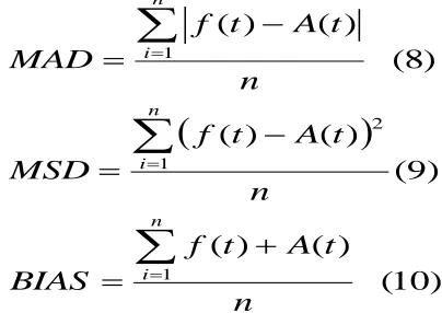
MAD = Mean Absolute Deviation MSD = Mean Squared Deviation A(t) = Actual data for t
f(t) = Predicted values for t
3. LEARNING CURVE MODEL
Various types of learning curve models are discussed below.
3.1 Power Model
This basic model was first described in 1936 by Theodore Paul Wright in the aircra ft industry as the first mathe matical mode l for learning [8]:
b
n
t
n
t
1
(1)
Where
100
(
2
)
bThis is a basic appro ximation of the lea rning phenomenon. It does not account for the smoothing of the curve, i.e . learning does not go on forever. Each time production is double the performance time is reduced by fraction b [1].
3.2 Arithmetic Model
This is the simplest method of modeling learning curves:
d n
t
t
1
(2)Implementation of Lean Manufacturing
Through Learning Curve Modelling for Labour
Forecast
Indra Gunawan
Department of Mechanical and Manufacturing Engineering Auckland University of Technology, Auckland, New Zealand
International Journal of Mechanical & Mechatronics Engineering IJMM E-IJENS Vo l:09 No:10 36 This model lac ks fle xib ility as production times can only be
determined for quantities doubled, i.e. 2, 4, and 8 [4]. Note the change of nomenclature in the equation for arith metic approach. This was to avoid confusion of para meters a mongst different models.
3.3 Cumulative Average Power Model
This model is based on the relationship between direct labour man-hours to the cumulative number of units produced:
b
n
t
n
t
1
^(3)
This model was developed by researchers when the regression value with the power model was unacceptably low. This model dampens out the ‘wild’ data points because it is a continually averaging process [1]. It has higher R2 values compared to the power model.
3.4 Stanford B Model
This is another modification of the Power model:
b
n
t
n
B
T
1
(
)
(4)
B is the experience factor of the operator (between 1 and 10) and a typical value of 4 is usually used. For small values of B th is model asymptotes fairly rap idly to the regular powe r model. Clearly this model was indented for use on learning curves of large products like aircrafts [1].
3.5 DeJong’s Learning Model
This model ta kes into account the manual and machine processing times. It includes an incompressibility factor (M ) for tasks that have machine co mponents. It is based on the fact that machine times do not increase and remain constant regardless of experience [1].
b
n
t
M
M
n
t
1
(
1
)
(5)Where M is the ratio of performance time a fter infinite cycles over performance time after 1st cycle (0 ≤ M ≤ 1). When there is no mach ine content M = 0.1 cyc les are required to reach the limit ing value. There has been no field data to support th is model.
3.6 Dar-El’s Modification of De Jong’s Model
The incompressibility factor is redefined as applying to all task ele ments. By ra ising the origina l powe r cu rve by A, a ne w learning curve line is created.
A
t
t
n
n
^
(6) This model e liminates the drawback of the power model in that it does not tend zero after an infinite number of repetitions.
3.7 Dar-El/Ayas/Gilad Dual Phase Model
This was generated when research data was poorly matched to all known mode ls. Prediction based on early data tends to underestimate and predict ions based on later data tend to overestimate. This poor fit occurred due to two separate types of lea rning occurring simultaneously, cognitive and motor learning.
Cognitive lea rning includes decision making, fo llo wing instructions, learning co mple x sequences, interpreting measurements, etc. This type of learning is much faster. Motor learning is a lot slower. It consists of the physical move ment required in order to co mplete a task (i.e. lowe r b value than cognitive).
Cognitive learn ing dominates initia lly, after wh ich motor learning dominates as the number of repetitions gets larger.
3.8 Bevis Towill Learning Model
This model uses an exponential law to show the output as a function of time. It has a ma ximu m leve l which is mo re realistic than the power model [1].
t
f c
t
R
R
e
R
1
(7)
Where τ = the time constant
This model is not practical to apply as the variables on which the model is based are hard to collect. For this reason there are
no applications of using this model.
4. CASE STUDY-COM PANY PRODUCTION Lean manufacturing is a technique that is commonly imple mented by production and project managers to improve productivity and reduce wastage. Metal Skills Ltd is one of New Zealand’s largest manufacturers of sheet metal products. Their customers inc lude US, Australian and Do mestics manufacturers. The objective of this study was to ultimately improve the company’s ability to meet deadlines. This was to be done through the learning curve mode lling for labour forecast.
In order to find specific models that can be applied to this company, data was required to be collected. The procedure followed was to get permission fro m the managing directors to observe the workers after it was cleared by the shop floor manager. Once this was done health and safety regulations needed to be exp lained and abided by. Finally permission was gained fro m the worke r be ing observed so that they would not feel singled out.
model chosen.
The required data was collected fro m the folding department as shown in Fig. 1. Th is department was selected for some of the following reasons: 1) This is one of the bottlenecks in the factory. The other bottleneck was the welding bay, but due to health and safety standards required, data collection would have been difficult, 2) It has more manual components than any other departments, except weld ing, 3) It is the most utilised department in the factory, 4) Requires careful scheduling as it has the largest number of worke rs than any other departments.When collecting data it was important that the first cycle time recorded was taken for the first cycle of that batch so that the n value was valid. Many sets of data were collected but three main batches were used for analysis.
Fig. 1. A Press Brake Machine
Using statistical analysis the accuracy of each mode l to each set
of data was calculated, where:
)
10
(
)
(
)
(
)
9
(
)
(
)
(
)
8
(
)
(
)
(
1 1
2 1
n
t
A
t
f
BIAS
n
t
A
t
f
MSD
n
t
A
t
f
MAD
n
i n
i n
i
Three sets of data are collected and the highlighted values as the most accurate data for that statistical measure are shown in Table I.
TABLE 1.
SUMMARY OF LEARNING CURVE MODELS
DATA 1
Pow er Model
Cum ulative Average
Model
Stanford B Model
De Jong's Learning Model
Arithm etic Approach
Dual Phase Model
96% 95% 97% 96% 96% 97% 84% 82% 99% 98% 89% 88%
MAD 1.50 1.59 1.54 1.88 1.64 1.89 1.78 1.62 1.60 1.66 2.04 1.95
MSD 3.61 4.41 4.00 6.05 4.65 5.33 4.84 4.28 4.39 6.10 6.77 7.77
BIAS 0.05 -1.02 -0.09 -1.55 -0.51 0.72 0.79 0.44 0.12 -1.66 0.51 -0.63
0.05 1.02 0.09 1.55 0.51 0.72 0.79 0.44 0.12 1.66 0.51 0.63
DATA 2
Pow er Model
Cum ulative Average
Model
Stanford B Model
De Jong's Learning
Model
Arithm etic Approach
Dual Phase Model
97% 98% 98% 97% 98% 97% 90% 85% 100% 99% 89% 88%
MAD 1.30 1.26 1.27 1.33 1.24 1.28 1.26 1.30 1.40 1.49 1.56 1.60
MSD 2.41 2.32 2.33 2.58 2.26 2.36 2.31 2.40 3.00 3.52 3.77 3.81
BIAS -0.16 0.09 -0.09 -0.42 0.03 -0.25 0.04 -0.19 0.20 -0.45 0.32 0.04
0.156 0.094 0.091 0.425 0.032 0.246 0.037 0.190 0.200 0.450 0.315 0.040
DATA 3
Pow er Model
Cum ulative Average
Model
Stanford B Model
De Jong's Learning
Model
Arithm etic Approach
Dual Phase Model
94% 93% 95% 96% 94% 93% 60% 55% 96% 97% 87% 88%
MAD 1.84 1.98 2.11 2.18 2.23 2.56 2.40 2.46 3.11 2.14 1.82 1.70
International Journal of Mechanical & Mechatronics Engineering IJMM E-IJENS Vo l:09 No:10 38
5. LIMITAT IONS AND SUMMARY OF
LEARNING CURVES
There are some limitations of using learning curves that a company need to be made aware of in order to make proper use of learning curves [4]:
Learning curves vary from one industry to
another and also between companies in the
same industry. So it is important that a
company’s own learning curve is developed
rather than just applying someone else’s.
Learning curves are based on the data collected
for times observed. So it is important that this
data is consistent and as accurate as possible.
To
maintain
accuracy
re-evaluation
is
necessary as times progress.
The learning curves developed for a company
are unique to that company and the personnel
employed at the time of the data collection. As
staff changes so will the learning curve.
Learning curves are only applicable to direct
labour and not for indirect labour and
materials.
Learning curves are also affected by resource
availability and changes in the process as well
as cultural changes.
Learn ing curve models are summa rized be low in Table II according to their advantages and limitations:
TABLE II
COMPARISON OF LEARNING CURVE MODELS
Fro m the eight models investigated only six were actually compared against data collected at the company. The Bevis/Towill model was exc luded as the parameters are difficult to obtain fro m fie ld data and there are no known e xa mples of this being used. Dar El’s modification to De Jong’s model was also exc luded as the time in motion tables appropriate for this company were not made available.
Data set 1 and 3 de monstrated the expected trend. The trend of
data collected in sample 2 was unexpected. A reason for the fluctuating times was that the actual cycle t ime was so sma ll that the human error g reatly affects the data. The other two samples had cycle times that were much longer so the human error made up a smaller component of the time.
In order to get as accurate as possible times to norma l production rates it was important that the workers we re comfo rtable being timed and that they were made a ware of the
Model Advantages Limitations
Power Model • Simple and easy to use
• Performance time approaches zero as number of repetitions becomes
large
Cumulative Average Model • Dampens out 'wild' data
points
• Smoothing masks important changes
Stanford B Model • Includes an experience
factor
• Intended for use in industries with
large products like aeroplanes • With small B values it is almost
identical to power model
DeJong's Learning Model
• Takes into account that machining time is not compressible with respect
to experience
• No field data to support this model
Dar-El's Modification to DeJong's Model
• Incompressibility factor redefined to apply
to all tasks • Eliminates the drawbacks
of power model
• When the number of repetitions is less than 150 the incompressibility
has no effect
Dual Phase Model
• Account for separate cognitive learning and motor learning rates
• Complex to apply • Requires electronic spreadsheet to
find parameters
Bevis/Towill Learning Model • Has a maximum learning
rate
• Great difficulty in finding the parameters to apply this model
reasons for the observations. Workers were timed for the end of a batch and then the data recorded was from the start of the next batch. This was done so that workers would be accustomed to the data
collector before the essential data was taken, thus reducing some of the error.
Using each model a p rediction was made using several different lea rning rates. Each of these was statistically compared to the actual data collected. Each set of data had different mode ls that were most accurate, but on the whole the power model was consistently one of the most accurate. Minimization of the MSD, MAD and BIAS we re done using solver to find the optimu m lea rning rate for each model. The most suitable learning curve rate was 96%.
6. CONCLUSION
A variety of learning curve models were considered and analysed. A learning curve has been identified to suit th e company’s production. This is the Power Model with a learning rate of 96%. Th is was selected as it is applicable to a wide range of production processes throughout the factory. The other models were re jected after analysis as they were found to be insufficient to the needs of the co mpany. The selected model was then validated against data collected in the factory and thus its application was justified. Application of this lea rning curve will better equip the company to manage job times and therefore be able to schedule more accurately and quoted due dates achieved with higher success rate.
REFERENCES
[1] Dar-El, E. (2000). Human Learning: From Learning Curves to Learning Organisations: Kluwer Academic Publisher.
[2] David A Nembhard, N. O. (2001). An Empirical Comparison of Forgetting Models. IEEE Transactions on Engineering Managem ent, 48(3), 283-291.
[3] Ebert, R. J. (1976). Aggregate Planning with Learning Curve Productivity. Management Science, 23(2), 171-182.
[4] Heizer, & Render. (2006). Operations Managem ent (8th ed.): Pearson Prentice Hall.
[5] Kaminsky, P., & Lee, Z.-H. (2008). Effective on-line algorithms for reliable due date quotation and large-scale scheduling. Journal of Scheduling, 11(3), 187-204.
[6] Shabtay, D., & Steiner, G. (2008). Optimal due date assignment in multi-machine scheduling environments. Journal of Scheduling, 11(3), 217-228.
[7] Walters, D. (2002). Operations Management-Producing Goods and Services (Second ed.). Essex: Pearson Education Limited.
[8] Wright, T. P. (1936). Factors affecting the cost of Airplanes. Journal of Aeronautical Sciences (3(4)), 122-128.