Learning Appropriate Contexts
Bruce Edmonds
Centre for Policy Modelling, Manchester Metropolitan University,
Aytoun Building, Autoun Street, Manchester, M1 3GH, UK. [email protected] http://www.cpm.mmu.ac.uk/~bruce
Abstract. Genetic Programming is extended so that the solutions being evolved do so in the context of local domains within the total problem domain. This produces a situation where different “species” of solution develop to exploit different “niches” of the problem – indicating exploitable solutions. It is argued that for context to be fully learnable a further step of abstraction is necessary. Such contexts abstracted from clusters of solution/model domains make sense of the problem of how to identify when it is the content of a model is wrong and when it is the context. Some principles of learning to identify useful contexts are proposed. Keywords: learning, conditions of application, context, evolutionary computing, error
1. Introduction
In AI there have now been many applications of context and context-like notions with a view to improving the robustness and generality of inference. In the field of machine learning applications of context-related notions have been much rarer and, when they do occur, less fundamental. Inductive learning, evolutionary computing and reinforcement techniques do not seem to have much use for the notion. There have been some attempts to apply context detection methods to neural networks, so that a network can more efficiently learn more than one kind of pattern but these have been limited in conception to fixes for existing algorithms.
absence of a good reason to do otherwise, to simplify things by combining the conditions of application of a model explicitly into the model content.
This paper seeks to make some practical proposals as to how notions of conditions of applicability and then contexts themselves can be introduced into evolutionary computing. Such a foray includes suggestions for principles for learning and identifying the appropriate contexts without prior knowledge.
2. Adding conditions of applicability to evolving models
2.1 Standard Evolutionary Computing Algorithms
Almost all evolutionary computing algorithms have the following basic structure: • There is a target problem;
• There is a population of candidate models/solutions (initially random);
• Each iteration some/all of the models are evaluated against the problem (either competitively against each others or by being given a fitness score);
• The algorithm is such that the models which perform better at the problem are preferentially selected for, so the worse models tend to be discarded;
• There is some operator which introduces variation into the population;
• At any particular time the model which currently performs best is the “result” of the computation (usually taken at the end).
There are various different approaches within this, for example, genetic programming (GP) (Koza, 1992). With GP the population of models can have a tree structure of any shape with the nodes and terminals taken from a fixed vocabulary. The models are interpreted as a function or program to solve the given problem, and usually given a numeric measure of their success at this – their “fitness”. The models are propagated into the next generation with a probability correlated to this fitness. The variation is provided by “crossing” the tree structures– as shown in figure 1).
Parent 1 Parent 2
Child 1 Child 2
For example, the problem may be that of finding a functional expression, e.g. 2
3
2
−
x
, to most closely “fit” a given set of data pairs. In this case the set of models will be trees with terminals being eitherx
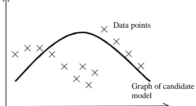
or a set of constants, the nodes might be the simple arithmetic operators, and the measure of success the inverse of the error of the resulting function with respect to the data.Data points
Graph of candidate model
Fig. 2. An illustration of a candidate functional “fit” for some data
One of the key features of such algorithms is that each candidate model in the population has the same scope – that of the problem. In the long run, a model can only be selected if it is successful (at least on average relative to other models) over the whole domain. Essentially the algorithm results in a single answer – the model that generally did best. There is no possibility that (in the long run) a model can be selected by doing well at only a small part of the whole problem. The technique is essentially context-free – the only context involved is that implied by the scope of the problem and that is selected manually by the designer.
2.2 Adding Conditions of Application
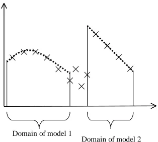
Domain of model 1
Domain of model 2
Fig. 3. Two models specialising in different parts of the problem.
It is well know that allowing “demes”, that is separate areas of evolution, acts to preserve the variety in the population. Allowing the problem space itself to structure the evolutionary should allow for clustering and competition according to what makes sense for that problem.
To do this each model in the population needs to indicate its conditions of application as well as its content, and both need to evolve in response to the problem presented within the problem domain. There are many different ways of doing this – perhaps the easiest is to simply position each model in the space and allow replication to other positions nearby.
One algorithm for this is:
Randomly generate candidate models and place them randomly about the domain, D
for each generation repeat
randomly pick a point in D, P
pick n models , C, biased towards those near P evaluate all in C over a neighbourhood of P pick random number x from [0,1)
if x < (1 – crossover probability)
then propagate the fittest in C to new generation
else cross two fittest in C, put result into new generation
until new population is complete
next generation
The idea is that models will propagate into the areas of the problem domain where they are relatively successful in (until a model that does even better locally appears).
The main parameters for this algorithm are: • Number of generations;
• Size of population;
• Number of models picked each tournament; • The extent of the bias towards the point, P, picked;
• The size of the neighbourhood that the models are evaluated over; • Probability of crossover.
Also, more importantly, the following need to be specified: • The problem;
• The language of the models in terms of their interpretation w.r.t. the problem (usually done in terms of nodes, and terminals if this is an untyped model);
• The space over which the models will propagate (usually a subspace of the domain of the problem).
A disadvantage of this technique is that once the algorithm has finished is does not provide you with a single best answer, but rather a whole collection of models, each with different domains of application. If you want a complete solution you have to analyse the results of the computation and piece together a compound model out of several models which work in different domains – this will not be a simple model with a neat closed form. Also there may be tough areas of the problem where ones does not find any acceptable models at all.
Of course, these “cons” are relative – if one had used a standard universal algorithm (that is all models having the same domain as the problem and evaluated over that domain), then the resulting “best” model might well not perform well over the whole domain and its form might be correspondingly more complex as it had to deal with the whole problem at once.
2.3 An Example Application
Fig. 4. The problem function – the number of sunspots
The fixed parameters were as follows: • Number of generations: 50; • Size of population: 723;
• Initial maximum depth of model: 5;
• Number of models picked each tournament: 6; • Locality bias: 10;
• Size of the neighbourhood: from 1 to 7 in steps of 2; • Probability of crossover: 0.1.
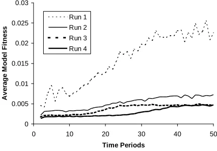
There were four runs, in each the neighbourhood over which the models were tested was 1, 3, 5, and 7 respectively. The first graph (Fig. 5) shows the average fitness of the models for these runs.
Fig. 5. The Average Fitness of Models in the four runs
0 5 0 0 1 0 0 0 1 5 0 0 2 0 0 0 2 5 0 0
0 5 0 1 0 0 1 5 0 2 0 0 2 5 0
T i m e P e r i o d s
Number of Sunspots
0 0.005 0.01 0.015 0.02 0.025 0.03
0 10 20 30 40 50
Time Periods
Average Model Fitness
The smaller the domain the greater the average model fitness. This is because it is much easier to “fit” an expression to a single point than “fit” longer sections of the graph, with fitting the whole graph being the most difficult. Of course, there is little point in fitting single points with expressions if there is not any generalisation across the graph. After all we already have an completely accurate set of expressions point-by-point: the original data set itself. On the other hand, if there are distinct regions of the problem space where different solutions make sense, being able to identify these regions and appropriate models for them would be very useful. If the context of the whole problem domain is sufficiently restricted (which is likely for most of the “test” or “toy” problems these techniques are tried upon).
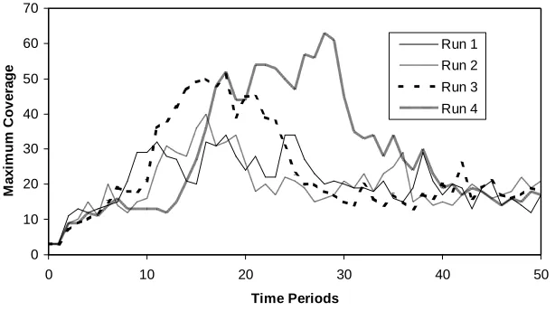
Figure 6, below, shows the maximum coverage of the models for the four runs. In each case early on a few models take over from the others in terms of the amount of problem space they occupy. Then as they produce descendants with variations, these descendants compete with them for problem space and the coverage of any particular model equals out.
Fig 6. Maximum coverage (in terms of number of positions) of models over the four runs
One individual propagates itself for a while before new models (often its own offspring) start to compete with it. This is illustrated in Fig. 7. Which shows the coverage of the dominant model at each stage of run four, where the different individual models are identified.
0 10 20 30 40 50 60 70
0 10 20 30 40 50
Time Periods
Maximum Coverage
Fig 7. Maximum coverage of individual models in fun 4 (the same individual is indicated by the same symbol and are connected)
Thus you get a short-term domination by individual models by propagation and a longer-term effect composed of the domination of closely related but different individuals – what might be called “species”. The end of run 4 is analysed below using a very rough division into such species. Those models that start with the same 25 characters are arbitrarily classed as the same species. The 10 most dominant species at the end of run 4 are shown below in Table 1.
Species Start of model Size of Domain
1 [ MINUS [ SAFEDIVIDE [ PLUS … 260
2 [ PLUS [ PLUS [ SIN [ TIMES … 187
3 [ PLUS [ SAFEDIVIDE [ PLUS … 31
4 [ MINUS [ MINUS [ x1] [ TIME ... 24 5 [ PLUS [ x1] [ SIN [ PLUS [ T … 22 6 [ PLUS [ MINUS [ x1] [ 0.641 ... 19
7 [ PLUS [ MINUS [ x1] [ 0.868 … 17
8 [ SAFEDIVIDE [ PLUS [ x1] [ … 13
9 [ MINUS [ MINUS [ x1] [ 0.57 … 12
10 [ PLUS [ PLUS [ SIN [ 0.5712 … 9
Table 1. The 10 “species” with the largest domain
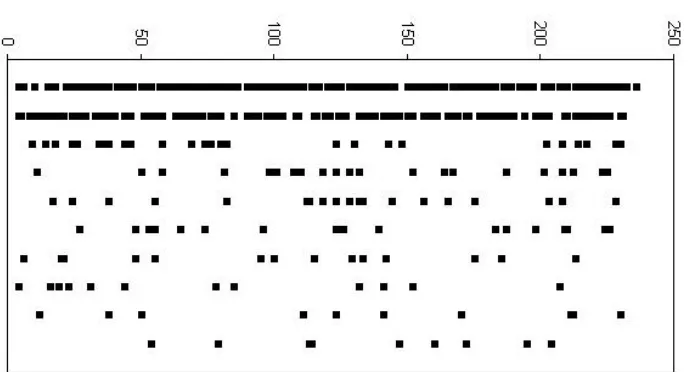
As you can see two quite different such “species” dominate. The figure below (Fig. 8.) Indicates the domains of these species.
0 10 20 30 40 50 60 70
0 5 10 15 20 25 30 35 40 45 50
Time Period
Fig. 8. The domains of the ten most common species (most dominant in the top line) of models at the end of run 4
Simply by inspection, some of these species do seem to have identifiable parts of the problem space in which they apply. This effect could be accentuated by adding a period of “consolidation” at the tail end of the algorithm. During this period there would be no crossover and the locality of the operation of the propagation process kept to a minimum. This would allow individual models to have a chance to “dominate” contiguous sub-spaces of the whole domain. Such a consolidation period has obvious parallels with the technique of “simulated annealing”, and I guess a similar technique of slowly lowering the “temperature” (the distance models can jump around) of the algorithm towards the end might have similar effects.
3. The move to really learning and using contexts
Given the picture of “context” as an abstraction of the background inputs to a model, implicit in the transfer of knowledge from learning to application (that I argued for in Edmonds, 1999). There is still a step to take in order for it to be truly “context” that is being utilised – a collection of conditions of application become a context if it is sensible to abstract them as a coherent unit. Now it may be possible for a human to analyse the results of the evolutionary algorithms just described and identify context – these would correspond to niches in the problem domain that a set of models competes to exploit – but the above algorithm itself does not do this.
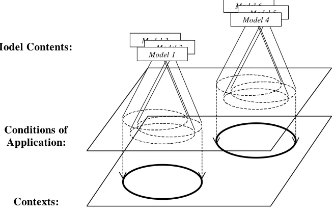
does when identifying the “niche” of an organism (or group of organisms) – this is not highly detailed list of where this organism happened to live, but a relevant abstraction from this taking into account the way the organism survives. This idea of abstracting a context from clusters of model domains is illustrated in Fig. 9. below.
Model 3 Model 2 Model 1
Model 6 Model 5 Model 4
Model Contents: Model Contents:
Conditions of Application:
Contexts:
Fig. 9. Contexts abstracted from models with different, but clustered, domains of application
Of course, it is not necessarily the case that the model domains will be clustered so that it is at all sensible to abstract them into explicit contexts. Rather this is a contingent property of the problem and the strategy, resources and limitations of the learner. The existence of meaningful contexts arises out of the fact that there happen to be heuristics that can do this clustering, otherwise even if all the relevant models are not universal in scope context, as such, might not arise.
4. Knowing whether it is the context or the content that is wrong
There is a fundamental difficulty is in attributing the source of error displayed by a model. Perhaps this, more than anything else, characterises different strategies for learning. Given that a model displays an unacceptable level of error in a situation, what are the options? They include:
1. Changing the model content (either by a minor elaboration or parameter adjustment or by a more radical restructuring);
2. Adjusting the conditions of application so as to exclude the domain where the model did not work;
3. Making the predictions of the model less precise so as to allow for the error; 4. Finally, and most radically it may be necessary to change the language/basis of
the model formulation itself.
The problem is to determine which is appropriate in each case. In this paper I am particularly focusing of the decision between (1) and (2) above (for a wider discussion see Moss and Edmonds 1998).
The point is that in isolation there is no principled way of telling whether it is the model content or context that is wrong. However, given that the problem or circumstances is such that there are meaningful clusterings of the domains of models into contexts there is a way, namely: to check the predictions of other models with the same context. If other models associated with the same context are also in error, then it is probably the context that is wrong; if the other models associated with the same context are correct then it is most likely the original model content that is in error. This collective view of model building suggests the following principles of context identification:
1. (Formation) A cluster of models with similar or closely related domains suggests these domains can be meaningfully abstracted to a context.
2. (Abstraction) If two (or more) contexts share a lot of models with the same domain, they may be abstracted (with those shared models) to another context. In other words, by dropping a few models from each allows the creation of a super-context with a wider domain of application.
3. (Specialisation) If making the domain of a context much more specific allows the inclusion of many more models (and hence useful inferences) create a sub-context.
4. (Content Correction) If one (or only a few) models in the same context are in error whilst the others are still correct, then these models should either be removed from this context or their contents altered so that they give correct outputs (dependent on the extent of modifications needed to “correct” them) 5. (Content Addition) If a model has the same domain as an existing context, then
add it to that context.
6. (Context Restriction) If all (or most) the models in a context seem to be simultaneously in error, then the context needs to be restricted to exclude the conditions under which the errors occurred.
8. (Context Removal) If a context has only a few models left (due to principle 2) or its domain is null (i.e. it is not applicable) forget that context.
These conditions are somewhat circular – context are guessed at from clusterings of model domains, and model contents are changed in models who disagree with a majority of models in the same context. However, I do think that these principles should allow the “bootstrapping” of meaningful contexts. A starting point for this process can be the assumption that models learnt in similar circumstances (situations) share the same context – that the relevant contexts are defined by the similarity of experience. Later these assumption based contexts can be abstracted, refined and corrected using the above. Any bootstrapping learning process depends upon the possibility of starting with simple models and situations and working upwards (compare Elman 1993).
5. Related Work
5.1 Evolutionary Computation
The obvious technique from evolutionary computation which employs ideas of model domains are Holland’s “Classifier” (Holland 1992) and descendent techniques. Here each model is explicitly divided into the conditions and action of a model. Such models are not designed to evolve in parallel as in the above algorithm, but to form computational chains.
Eric Baum has developed this idea by applying more rigorous property rules to govern the chaining of models and the apportionment of reward. Thus in his model each model has an implicit domain, in that it is only applies when it out-bids other models in order to be applied (Baum and Durdanovic, 2000b). In the most recent version of his algorithm (called Hayek 4) he also introduces explicit conditions of application as each model is a Post production rule (Baum and Durdanovic, 2000a).
5.2 Machine Learning
Peter Turney surveys the various heuristics tried to mitigate the effects of context on machine learning techniques in (Turney 1996). He keeps an extensive bibliography on context-sensitive learning at URL:
http://extractor.iit.nrc.ca/bibliographies/context -sensitive.html
6. Conclusion
If one abandons the myopic view of focusing on single model solutions and models, and looks at their group dynamics instead, then further learning heuristics become available. These allow one to distinguish when it is the identification of the content or the context that is at error. Indeed it is only by considering groups of models that contexts themselves make any sense.
7. References
Aha, D. W. (1989). Incremental, instance-based learning of independent and graded concept descriptions. In Proc. of the 6th Int. Workshop on Machine Learning, 387-391. CA: Morgan Kaufmann.
Baum, E. and Durdanovic, I. (2000a). An Evolutionary Post-Production System.
http://www.neci.nj.nec.com/homepages/eric/ptech.ps
Baum, E. and Durdanovic, I. (2000b). Evolution of Co-operative Problem Solving.
http://www.neci.nj.nec.com/homepages/eric/hayek32000.ps
Edmonds, B. (1990). The Pragmatic Roots of Context. CONTEXT'99, Trento, Italy, September 1999. Lecture Notes in Artificial Intelligence, 1688:119-132.
Elman, J. L. (1993). Learning and Development in Neural Networks - The Importance of Starting Small. Cognition, 48:71-99.
Gigerenzer, G and Goldstein, D. G. (1996). Reasoning the fast and frugal way: Models of bounded rationality. Psychological Review, 104:650-669.
Harries, M. B., Sammut, C. and Horn, K. (1998). Extracting Hidden Contexts. Machine Learning, 32:101-126.
Holland, J. H. (1992). Adaptation in Natural and Artificial Systems, 2nd Ed., MIT Press, Cambridge, MA.
Koza, J. R. 1992. Genetic Programming: On the Programming of Computers by Means of Natural Selection. Cambridge, MA: MIT Press.
Moss, S. and Edmonds, B. (1998). Modelling Economic Learning as Modelling. Cybernetics and Systems, 29:215-248.
Turney, P. D. (1993). Exploiting context when learning to classify. In Proceedings of the European Conference on Machine Learning, ECML-93. 402-407. Vienna: Springer-Verlag. Turney, P. D. (1996). The management of context-sensitive features: A review of strategies. Proceedings of the ICML-96 Workshop on Learning in Context-Sensitive Domains, Bari, Italy, July 3, 60-66.
Turney, P. D. and Halasz, M. (1993). Contextual normalisation applied to aircraft gas turbine engine diagnosis. Journal of Applied Intelligence, 3:109-129.