Compton Scattering on Light Nuclei
Deepshikha Shukla1,a
The University of North Carolina, Chapel Hill, North Carolina, USA.
Abstract. Compton scattering on light nuclei (A = 2,3) has emerged as an effective avenue to search for signatures of neutron polarizabilities, both spin–independent and spin–dependent ones. In this discussion I will focus on the theoretical aspect of Compton scattering on light nuclei; giving first a brief overview and therafter concentrating on our Compton scattering calculations based on Chiral effective theory at energies of the order of pion mass. These elasticγd andγHe-3 calculations include nucleons, pions as the basic degrees of freedom. I will also discussγd results where the∆-isobar has been included explicitly. Our results on unpolarized and polarization observables suggest that a combination of experiments and further theoretical efforts will provide an extraction of the neutron polarizabilities.
1 Introduction
Neutron structure is governed by strong-interation dynam-ics and hence its electromagnetic properties encode infor-mation that contribute to our understanding of Quantum ChromoDynamics (QCD). For example, an early success of the S U(3) quark picture was its prediction of magnetic moments,µ, for the neutron and other strongly-interacting particles (hadrons). Magnetic moments are a first-order re-sponse to an applied magnetic field. In this discussion how-ever, the focus is on electromagnetic polarizabilities. The two most basic polarizabilities are the electric and mag-netic ones,αE1andβM1, which quantify the second-order response of an object to electric or magnetic field (that pro-duces an induced dipole moment). The Hamiltonian for a neutral particle (in this case, a neutron) in applied electric and magnetic fields,EandB, is then:
H=−µ·B−2πhαE1(ω)E2+βM2(ω)B2
i
. (1)
Eq. (1) contains terms that are quadratic in the applied electromagnetic field. If we now consider the derivatives (first-order) of the applied fields, four new structures ap-pear which are second order inEandB [1] and are ex-plicitly dependent on the intrinsic spin of the object. They are:
−2πhγE1E1σ·E×E˙+γM1M1σ·B×B˙ −2γM1E2σiEi jBj+2γE1M2σiBi jEj
i
(2)
with Ti j :=12(δiTj+δjTi). The coefficientsγ...s are the so-called “spin polarizabilities”. Eqs. (1) and (2) encode the multipole parameterizations of the polarizabilities and any other representation of the polarizabilities (for instance, spin polarizabilitiesγ1–γ4) can be expressed as linear
com-binations of these polarizabilities. This discussion intends
a e-mail:[email protected]
to show that for the neutron, these six polarizabilities can be extracted from Compton scattering on on the deuteron and3He.
Polarizabilities such as those in Eqs. (1) and (2) can be accessed in Compton scattering because the effective Hamiltonian yields a nucleon Compton scattering ampli-tude of the form:
TγN =
X
i=1...6
Ai(ω, θ)ti. (3)
Here t1–t6 [2] are invariants constructed out of the
pho-ton momenta and polarization vectors (ˆǫand ˆǫ′). t1and t2
contain terms that are nucleon-spin independent whereas
t3–t6 include nucleon spin. The Ai’s are Compton
struc-ture functions; expanding these Aiaroundω=0 illustrates the how the polarizabilities affect the Compton amplitude. α β enter atO(ω2) whereas the spin-polarizabilities enter at O(ω3). For the proton, the Thomson term, −Q3
Mǫˆ ′·ǫˆ ensures a larger cross section (compared to the neutron) and from low-energy Compton scattering measurements α(p)andβ(p)can be extracted. A combined analysis of the differential cross-sections (dcs) of a number ofγp experi-ments over the past decade [3] yields the PDG values:
αp =(12.0±0.6)×10−4fm3,
βp =(1.9±0.5)×10−4fm3. (4)
Similar extractions for the neutron is not possible be-cause
– the neutron Thomson term is absent and,
– there are no free-neutron targets as neutrons are very short-lived (lifetime∼880 secs.).
Of all the possible ways to access neutron polarizabilities (that includes scattering neutrons offa heavy nucleus such as lead), Compton scattering on light nuclei has emerged as likely candidates that would enable the extraction of the
DOI:10.1051/epjconf/20100304001
six neutron polarizabilities. For instance, the latest global analysis of the 28 points for deuteron Compton scattering gave
αs=11.3±0.7stat±0.6Baldin±1th
βs=3.2∓0.7stat±0.6Baldin±1th (5)
for the iso-scalar nucleon polarizabilities [4, 5] with the Baldin sum rule ¯α(s) +β¯(s) = 14.5±0.6 as constraint.
The situation for the neutron spin polarizabilities is much worse and the only data available are for the forward and the backward spin polarizabilities, which are linear combi-nations of the four spin polarizabilities. The neutron back-ward spin polarizability was determined to be
γπ =−γE1E1−γE1M2+γM1E2+γM1M1
=(58.6±4.0)×10−4fm4, (6)
from quasi-free Compton scattering on the deuteron [6]. TheχPT prediction forγπis 57.4×10⁻⁴fm4[7]. The
for-ward spin polarizability,γ0, is related to energy-weighted
integrals of the difference in the helicity-dependent pho-toreaction cross-sections (σ1/2−σ3/2). Using the optical
theorem one can derive the following sum rule [2, 8]:
γ0 =−γE1E1−γE1M2−γM1E2−γM1M1
= 1 4π2
Z ∞
ωth
σ1/2−σ3/2
ω3 dω, (7)
whereωthis the pion-production threshold. The following results onγ0were obtained using the VPI-FA93 multipole
analysis [9] to calculate the integral on the RHS of Eq. (7):
γ0≃ −0.38×10⁻⁴fm4. (8)
TheχPT prediction forγ0is consistent with zero [7].
New data for unpolarized deuteron Compton scattering from MAXlab is being analysed [10], and an experiment at HIγS is approved. Additionally, the fact that a polarized
3He nucleus behaves as an effective neutron [11] has
gen-erated interest in3He Compton scattering. The first elas-tic γ3He calculations were reported in Ref. [12–14] and preparations are underway for a proposed experiment at HIγS. Currently, a concerted effort is underway to reduce the theory-error using higher orders in the chiral count-ing [15]. The goal is a comprehensive approach to Comp-ton scattering in the proComp-ton [16, 17], deuteron [4, 5, 16, 18– 20] and3He [12–14] inχEFT from zero energy to beyond
the pion-production threshold. These proceedings give a quick overview of the current investigations to help extract the neutron polarizabilities from polarized and unpolarized deuteron and3He Compton scattering.
2 Compton scattering off a nucleon
In order to calculate the Compton amplitude (3) at energies of the order of the pion mass, we employ Heavy Baryon Chiral Perturbation Theory (HBχPT ) with pions and nu-cleons as effective degrees of freedom [2]. The expansion
parameter in this formulation is Q =
p,mπ
M,Λχ
, where p is a small momentum usually comparable to the pion mass,
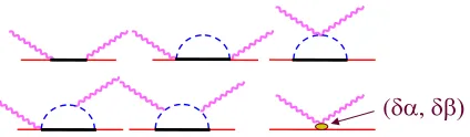
mπ; M is the nucleon mass and Λχ is the scale of chiral symmetry breaking. Fig. 1 shows the leading and the next-to-leading order contributions in this framework. At this order the theory is parameter-free and the polarizabilities are then predictions of the theory. The nucleon Compton
LO
NLO
Fig. 1.The LO and NLO contributions to nucleon Compton scat-tering. The wiggly lines are photons, dashed ones are pions and the solid ones are nucleons. Permutations and crossed diagrams not shown.
amplitude at NNLO has also been calculated [21], however for the purpose of the results reported in these proceedings they are immaterial.
(
GD
,
GE
Fig. 2.The∆contributions to nucleon Compton scattering up to NLO. The thick solid ones are depict the intermediate∆-isobar.
The∆-isobar can be included explicitly in the calcula-tion and the results reported in these proceedings employ the “Small Scale Expansion” (SSE) scheme [22]. In this scheme the expansion parameter,εdenotes either a small momentum, the pion mass, or the mass difference∆0
be-tween the real part of the ∆mass and the nucleon mass,
3 The nucleon inside a nucleus
Theγ-nucleus scattering amplitude is written as
M=hΨf|Oˆ|Ψii, (9)
with|Ψiiand|Ψfibeing the nuclear wavefunctions. ˆO rep-resents the photon-nucleon(s) interaction kernel that is cal-culated usingχPT . The nuclear wavefunctions are usually derived from a potential model or a chiral potential.
Neutron properties are usually extracted from data taken on few-nucleon systems by dis-entangling nuclear-binding effects. Within the power-counting scheme used for these calculations, these effects include pion-exchange mecha-nisms between two nucleons at the lowest order (see Fig. 3). The external photon may either couple to a pion-nucleon vertex or an exchanged pion. The graphs shown in Fig. 3 enter theγd orγ3He calculation only at next-to-leading
or-der (O(Q3)). Additional contributions at NNLO have also
Fig. 3. Lowest-order two-body current contributions. They enter aγ-nucleus calculation at NLO. Crossed graphs and graphs with the nucleons interchanged are not shown.
been calculated [16] but are not essential for this discus-sion.
4 Observables
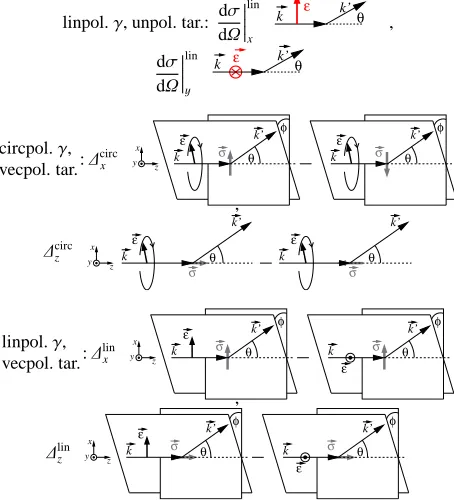
The availability of polarized beams and the technology to polarize targets has opened up the field of possible mea-surements. Over and above the canonical differential cross-section, one can now measure observables that include dif-ferent combinations of unpolarized/polarized beam and tar-get. Fig. 4 gives a representation of the observables consid-ered. The convention adopted is that the beam direction is the z-axis and the x−z plane is the scattering plane. For
a linearly polarized beam and unpolarized target, ddσΩ lin
x is the differential cross-section for photon polarization in the scattering plane, and ddσΩ
lin
y for perpendicular polariza-tion. The∆s are the double polarized observables that in-volve a vector-polarized deuteron and a circularly or lin-early polarized photon.∆circx(z)gives the difference in the dif-ference in the differential cross-sections between config-urations when the target is polarized along +ˆx (+ˆz) and −ˆx (−ˆz) using a circularly polarized beam.∆linx(z)gives the photon polarization asymmetry when the target is polar-ized along+ˆx (+ˆz). Experimental measurents often use the asymmetriesΣobtained by dividing the∆s by the sum of the measured differential cross-sections. Of course, these asymmetries are then devoid of systematic uncertainties.
linpol.γ, unpol. tar.: dσ dΩ
lin
x ε
k k’θ ,
dσ
dΩ
lin
y
k ε k’θ
circpol.γ, vecpol. tar.:∆
circ x
x y
z
k’ σ
ε k’
σ
ε
k
k θ θ
φ φ
,
∆circ z
ε
k’
σ k
z x y
ε
k’
k
σ θ θ
linpol.γ, vecpol. tar.:∆
lin x
k’ σ
k’ σ k k
ε x y z
ε
θ θ
φ φ
,
∆linz
k’ σ
k’ σ k k
ε x y
z
ε
θ θ
φ φ
Fig. 4.Definition of observables for singly and double polarized observables. Figure from H. Grießhammer.
The observables described above are only a subset of all the possible combinations. The focus of these proceed-ings is only on some prominent examples. For the deuteron, representative results for most of the above obervables are presented. The aim is to aid in planning new experiments, and the results for all of the above observables are available as an interactive Mathematica 7.0 notebook from Grießham-mer ([email protected]). For the3He Compton scattering cal-culation results for the unpolarized differential cross-section and∆circ
x(z)only are presented.
5 Elastic
γ
d scattering
The NLO (O(ε3)) deuteron Compton scattering
calcula-tions in the SSE variant ofχPT include the amplitudes of Secs. 2 and 3. Note that the pion-pole graph of Fig. 1 does not contribute to deuteron Compton scattering as deuteron is an isoscalar. There is an additional ingredient in the calculation – resumming the intermediate NN-rescattering states. A consistent description ofγd Compton scattering must also give the correct Thomson limit, an exact low-energy theorem which in turn follows from gauge invari-ance [23]. In deuteron Compton scattering, this mandates the inclusion of TNN whenever both nucleons propagate close to their mass-shell between photon absorption and emission, i.e. when the photon energyω . 50 MeV. At higher photon energiesω&60 MeV, the nucleon is kicked far enough offits mass-shell, E ∼Q, for the amplitude to
Fig. 5. Low-energy NN rescattering contributions to deuteron Compton scattering. The rectangle in the middle represents the
NN T-matrix.
Once all the ingredients in ˆO of Eq. (9) are
deter-mined, it is folded with deuteron wavefunctions to obtain the deuteron Compton amplitude, using which any observ-able can be calculated. For the results reported here we use chiral NNLO wavefunctions for the deuteron and the
AV18 potential in the intermediate NN-rescattering
pro-cess. While it is desirable that for a consistent calcula-tion theγNN kernel, the wavefunctions and the potential
used to calculate the intermediate rescattering contribution should be derived using the same framework. Our γNN
kernel and the wavefunctions are indeed derived from the same framework, but AV18 is not a chiral potential. How-ever, it has been shown in Ref. [4] and since then we have verified that the form of the potential used in the interme-diate rescattering process causes barely perceivable diff er-ence in the final results. Issues of matching currents and couplings etc. only appear at two higher orders than what we calculate.
Also note that the polarizabilities extracted from deuteron Compton scattering are the isoscalar combina-tions. This means that the extraction of the neutron izabilities will depend on how accurately the proton polar-izabilities are known.
5.1 Significance of the∆andNNRescattering on Polarization Observables
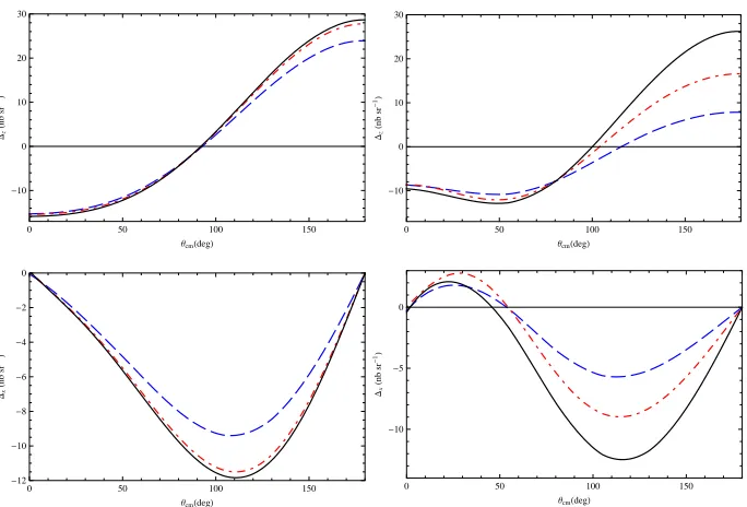
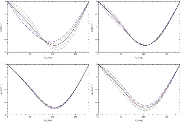
We first analyse the impact of including the∆-isobar and intermediate NN rescattering contributions on polarization observables. Figure 6 compares double-polarization observ-ables within different schemes. The top row shows ∆circ
z (left: 45 MeV and right: 125 MeV) and the bottom row shows∆circx (left: 45 MeV and right: 125 MeV). In the left-hand panels, the dashed line is aO(Q3) HBχPT calculation without dynamical∆or rescattering, the dot-dashed line is the same calculation with NN-rescattering included, and the solid line is aO(ε3) calculation with both intermediate
NN rescattering and a dynamical∆. In the right-hand pan-els, the dashed line is aO(Q3) HBχPT calculation with-out dynamical∆, the dot-dashed line has the dynamical ∆added, but no NN-rescattering, and the solid line is the full calculation with intermediate NN rescattering and a dynamical∆ As for unpolarized observables [5, 19], the ∆(1232) does not contribute appreciably at 45 MeV, but the observable is still ruled by including intermediate NN rescattering for the correct Thomson limit. In contrast, the ∆and intermediate NN-rescattering are equally significant at 125 MeV.
Thus, together with the observations of Refs. [5, 19] for unpolarized deuteron Compton scattering, we emphasize
that the ∆-isobar and the intermediate NN- rescattering contributions are necessary ingredients of our calculations that attempt to identify observables for the extraction of neutron polarizabilities in the energy range 45 – 125 MeV (lab). It has been verified that the dependence on the poten-tial that is used to generate the deuteron wavefunctions and the NN T-matrix (in the intermediate state) is negligible.
5.2 Results
0 30 60 90 120 150 180
Θdeg
20 21 22 23 24 25 26
d
Σ
d
y
lin
nbarn
sr
Ωlab45 MeV,∆ΑE1 2,∆ΒM1 2
0 30 60 90 120 150 180
Θ@degD
6 8 10 12 14 16 18
@
d
Σ
d
W
Dy
lin
@
nbarn
sr
D
Ωlab=125 MeV,∆ΑE1= ±2,∆ΒM1= ±2
0 30 60 90 120 150 180
Θdeg
6 8 10 12 14 16
d
Σ
d
y
lin
nbarn
sr
Ωlab125 MeV,∆ΓM1M1 2
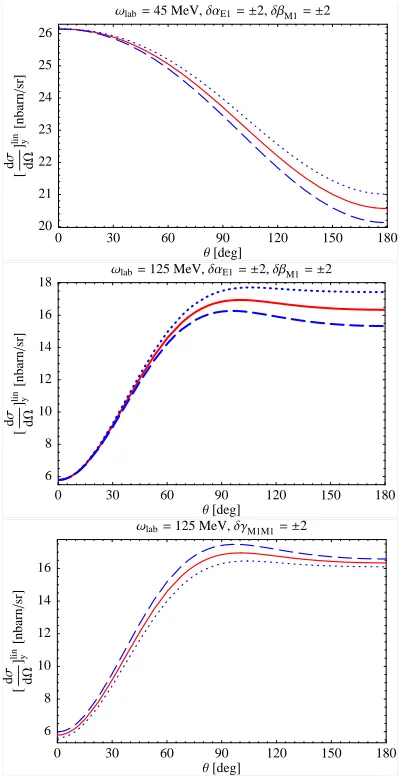
Fig. 7. Differential cross-sections with photons linearly-polarized along they-axis. Top and middle panels: The combi-nation αE1 −βM1 is varied, while their sum is constrained by
the Baldin sum rule. Bottom panel:γM1M1varied by±2 units at
ωlab=125 MeV.
0 50 100 150
10 0 10 20 30
Θcmdeg
z
nb
sr
1
0 50 100 150
10 0 10 20 30
Θcmdeg
z
nb
sr
1
0 50 100 150 -12
-10 -8 -6 -4 -2 0
ΘcmHdegL Dx
H
nb
sr
-1L
0 50 100 150 -10
-5 0
ΘcmHdegL Dx
H
nb
sr
-1L
Fig. 6.Effects of∆(1232) and of resumming NN intermediate states on the double polarization observables∆z(top) and∆x(bottom).
Left:ωlab=45 MeV; right:ωlab=125 MeV. Legend given in the text. 2
have adopted the strategy whereby we arbitrarily add six parametersδαE1,δβM1andδγi js to the calculation to repre-sent effects not explictly included in the theory. This allows us to gauge the dependence of the observables on these pa-rameters.
The topmost panel of Fig. 7 shows ddσΩ
lin
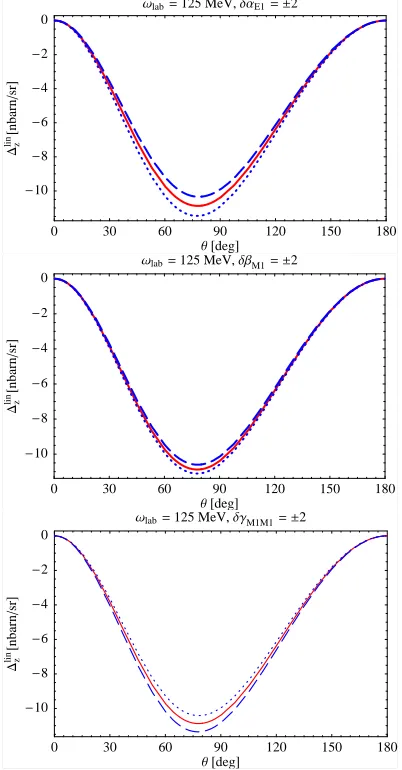
y at 45 MeV (lab). At this energy, there is appreciable sensitive only to αE1andβM1. At 125 MeV (lab) (middle and bottom pan-els) however, the sensitivity toγM1M1 is large and compa-rable to that ofαE1−βM1. Note that the sensitivity toγM1M1 decreases at back angles where the sensitivity toαE1−βM1 is largest. Fig. 8 shows the double-polarization observable ∆lin
z at ωlab =125 MeV. There is comparable sensitivity
to three of the polarizabilitiesαE1,βM1andγM1M1. Finally, we show the double-polarization observable∆circ
x atωlab=
125 MeV in Fig. 9. There is appreciable and comparable sensitivity toαE1,βM1andγE1E1, but only minor sensitiv-ity to the other spin-polarizabilities.
The other observables (not shown here) also show mi-nor sensitivity to some of the polarizabilities. The message to take away from this analysis is that no obervable is sen-sitive to only one of the polarizabilities. Ideally, the extrac-tion of the six polarizabilities should be performed from a global fit to a number of experimental measurements. Practically however, one should be judicious in selecting suitable observables for the extraction the polarizabilties. Configurations can be isolated where the contribution of one (or more) of the polarizabilities is zero. For example, see Fig. 10 where a detector under 90◦can therefore not de-tect M1 photons radiated from the induced magnetic dipole in the nucleon, cf. [24].
Also note that the sensitivity toαE1andβM1manifests at much lower energies (see for e.g. Fig. 7 and 10) com-pared to the spin polarizabilities. It is therefore advisable
to focus on αE1 andβM1 at lower energies and the spin polarizabilities at higher energies. It is imperative that the values of the electric and magnetic polarizabilities be bet-ter extracted so as not to taint any extraction of the spin polarizabilities.
6 Elastic
γ
3He scattering
This section reports calculations for3He Compton scatter-ing atO(Q3) in HBχPT . The operator ˆO in Eq. (9) is the
irreducible amplitude for elastic scattering of real photons from the NNN system. AtO(Q3) this operator encodes the
physics of two photons coupling to a two-nucleon system inside the3He nucleus. We do not have to include any ir-reducible three-body Compton mechanisms in our calcu-lation because they appear at the earliest at O(Q5). This
allows us to treat the3He nucleus as a (2+1) nucleon
sys-tem and enables the simplification of Eq. (9) to:
M=3hΨf| 1 2
ˆ
O1B(1)+Oˆ1B(2)+Oˆ2B(1,2)|Ψii, (10)
using the Faddeev decomposition of |Ψi. The struc-ture of the calculation is then similar for the one- and two-body parts. The superscript 1B in ˆO1B(a) of Eq. (10)
refers to the one-body mechanisms or the γN amplitude where the external photon interacts with nucleon ‘a’ (refer to Fig. 1). Similarly, ˆO2B(a,b) represents two-body
mech-anisms where the external photons interact with the pair ‘(a,b)’ (refer to Fig. 3).
0 30 60 90 120 150 180
Θdeg
12
10
8
6
4
2 0 2
x
circ
nbarn
sr
0 30 60 90 120 150 180
Θdeg
12
10
8
6
4
2 0 2
x
circ
nbarn
sr
Ωlab125 MeV,∆ΓM1M1 2
0 30 60 90 120 150 180
Θdeg
12
10
8
6
4
2 0 2
x
circ
nbarn
sr
Ωlab125 MeV,∆ΓE1M2 2
0 30 60 90 120 150 180
Θdeg
12
10
8
6
4
2 0 2
x
circ
nbarn
sr
Ωlab125 MeV,∆ΓM1E2 2
Fig. 9. The double-polarization asymmetry∆circ
z with circularly-polarized photons atωlab =125 MeV. From top left to bottom right,
variation by±2 units ofαE1,βM1,γE1E1,γM1M1,γE1M2,γM1E2.
scattering calculations are the first such calculations. In future, we intend to extend these calculations to include: the next higher order interactions, the∆-isobar as an ex-plicit degree of freedom and also the effects of intermedi-ate NNN-rescattering.
6.1 Results
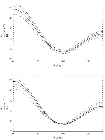
The amplitude (10) is now used to calculate observables. In Fig. 11 we plot ourO(Q3) differential cross-section
pre-dictions for elastic γ3He scattering. The two panels are
forω =60 and 120 MeV. Both show three different dcs calculations—O(Q2):dashed curve, IA (Impulse Approx-imation): dot-dashed curve and O(Q3): solid curve. The O(Q2) calculation includes only the proton Thomson term,
since that is the LOγN amplitude inχPT at that order. The
IA calculation contains only one-bodyO(Q3) contribution
(graphs in Fig. 1. There is a sizeable difference between the
IA and the O(Q3) confirming that two-body currents are equally important. Also, the difference betweenO(Q3) and
O(Q2) is very small at 60 MeV—showing thatχPT may
converge well there. This difference gradually increases with energy which may be partly because the fractional effect of the polarizabilities increases withω.
To analyze the effect ofαandβon the dcs, in Fig. 12 we plot theO(Q3) dcs at 80 MeV obtained when we add
shifts,∆α(n) and∆β(n), to theO(Q3) values ofαandβfor the neutron (see for e.g Ref. [2]). ∆α(n) is varied in the range (−4. . .4)×10−4fm3(long-dashed curve . . . dashed
curve) in steps of 2×10⁻⁴ fm3. Similarly,∆β(n) between
(−2. . .6)×10−4fm3(long-dashed curve . . . dashed curve)
in steps of 2×10⁻⁴fm3. This assesses the impact that one
set of higher-order mechanisms has on ourO(Q3) predic-tions. Notice that the sensitivity toβ(n)vanishes atθ=90◦. This is because α(n) andβ(n) enter A(n)
1 in the
combina-tionα(n)+β(n)cosθ. This implies thatα(n) andβ(n)can be
extracted independently from the same experiment. Sec-ondly, the absolute size of the shift in the dcs due to∆α(n)
and∆β(n)is roughly the same for all energies. This suggests
that measurements could be done atω ≈80 MeV, where the count rate is higher, and the contribution of higher-order terms in the chiral expansion should be smaller. Thirdly, the sequence of the curves for different values of ∆β(n)reverses if one compares the forward and backward
angles. This suggests that a meaurement of the forward to back angle ratio of the dcs will enhance the effect of∆β(n). Before examining double-polarization observables in γ3He scattering we try to develop some intuition for the
γ3He amplitude.3He is a spin-1
2 target – this means that
the matrix element (10) can be decomposed in the same fashion as the nucleon’s Compton matrix element in Eq. (3).
Tγ3He=
X
i=1...6
A3iHe(ω, θ)ti; Ai3He=A1Bi +A2Bi , (11)
where A1B
i (A
2B
i ) comes from considering the matrix el-ement of the one-body (two-body) operators in Eq. (10). The structures t3–t6now involve the ‘nuclear’ spin. In the
ground state of polarized3He, the two proton spins are
anti-aligned for the most part, therefore the nuclear spin is largely carried by the unpaired neutron [11]. We find that theO(Q3) two-body currents A2B1 and A2B2 are numer-ically sizeable, but A2B3 –A2B6 are negligible. Hence, to the extent that polarized3He is an ‘effective neutron’, we ex-pect A3iHe = A(n)i for i = 3–6. Thus, it is possible to look for the effects of the ‘neutron’ spin polarizabilities directly in a polarized3He Compton scatteing experiment.
More-over, since A3He
1 is dominated by the two proton
Thom-son terms, we anticipate a more enhanced signal from the neutron spin polarizabilities than is predicted for the corre-spondingγd observables (see Sec. 5.2 and Refs. [20, 25]).
0 50 100 150 -15
-10 -5 0 5 10 15
ΘcmHdegL Dz
I
nb
sr
-1M
0 50 100 150 -15
-10 -5 0 5 10 15
ΘcmHdegL Dz
I
nb
sr
-1M
0 50 100 150 -15
-10 -5 0 5 10 15
ΘcmHdegL Dz
I
nb
sr
-1M
0 50 100 150 -15
-10 -5 0 5 10 15
ΘcmHdegL Dz
I
nb
sr
-1M
Fig. 13. ∆circ
z atωcm=120 MeV withγ(n)1 (top left)–γ (n)
4 (bottom right) varied one at a time. The spin polarizabilities are varied by±100%
of theirO(Q3) values [2].
0 50 100 150 -8
-6 -4 -2 0
ΘcmHdegL
Dx
I
nb
sr
-1M
0 50 100 150 -8
-6 -4 -2 0
ΘcmHdegL
Dx
I
nb
sr
-1M
0 50 100 150 -8
-6 -4 -2 0
ΘcmHdegL
Dx
I
nb
sr
-1M
0 50 100 150 -8
-6 -4 -2 0
ΘcmHdegL
Dx
I
nb
sr
-1M
Fig. 14. ∆circ
x (c.m. frame) atωcm=120 MeV whenγ1(n)(top left)–γ (n)
4 (bottom right) are varied one at a time. The spin polarizabilities
are varied by±100% of theirO(Q3) values [2].
3He wave function is obtained by solving the Faddeev
equations with NN and 3N potentials derived fromχPT. All of the effects due to neutron depolarization and the spin-dependent pieces of ˆO2B are included in our calcu-lation of the amplitude (9). This yields the results for∆circz
and ∆circ
combi-0 30 60 90 120 150 180
Θ@degD
-10
-8
-6
-4
-2
0
Dz
lin
@
nbarn
sr
D
0 30 60 90 120 150 180
Θ@degD
-10
-8
-6
-4
-2
0
Dz
lin
@
nbarn
sr
D
Ωlab=125 MeV,∆ΒM1= ±2
0 30 60 90 120 150 180
Θdeg
10
8
6
4
2 0
z
lin
nbarn
sr
Ωlab125 MeV,∆ΓM1M1 2
Fig. 8. The double-polarization observable ∆lin
z with
linearly-polarized photons atωlab = 125 MeV. αE1 (βM1) is varied by ±2 units in the topmost (middle) panel. The bottom panel shows variation ofγM1M1by±2.
nations of the multipole parameterizations of Eq. (2).) In both Fig. 13 and Fig. 14 the∆γ(n)1 . . . ∆γ4(n)(top left to bot-tom right) are varied one by one by±100% of theirO(Q3)
predicted values [2]. Both∆circ
z and∆circx are quite sensitive toγ(n)1 , γ2(n), andγ(n)4 – ∆circ
z seems to be sensitive to the combinationγ(n)1 −(γ(n)2 +2γ4(n)) cosθwhereas∆circ
x is sensi-tive to a different one. With the expected photon flux at an upgraded HIγS such effects can be measured [26]. Notice that two different linear combinations ofγ(n)1 ,γ2(n), andγ(n)4 can be extracted through measurements at different angles. For a more detailed discussion see [12, 14]. Thus,∆circ
z and
∆circx are sensitive to two different linear combinations of γ(n)1 ,γ(n)2 , andγ(n)4 and their measurement should provide an unambiguous extraction ofγ(n)1 , as well as constraints onγ2(n)andγ4(n).
0 30 60 90 120 150 180
Θdeg
21 22 23 24 25 26
d
Σ
d
y
lin
nbarn
sr
Ωlab45 MeV,∆ΑE1 2
0 30 60 90 120 150 180
Θdeg
21 22 23 24 25 26
d
Σ
d
y
lin
nbarn
sr
Ωlab45 MeV,∆ΒM1 2
Fig. 10.Plots ofhdσ dΩ
ilin
y atωlab=45 MeV with varyingαE1(top)
and βM1 (bottom).Notice that the sensitivity toβM1 vanishes at
90 deg.
7 Summary and Outlook
Results of elastic deuteron and 3He Compton scattering
have been presented with the aim of extracting neutron polarizabilities. Our results show that most of the observ-ables are quite sensitive to the polarizabilities. The elec-tric and magnetic polarizabilities can also be directly ex-tracted from the unpolarized deuteron Compton scattering dcs (as shown in Refs. [4, 5, 16]) and unpolarized dcs mea-surements are underway at MAXLab in Sweden [10]. It is essential to accurately know the values of the electric and magnetic polarizabilities before focussing on the spin po-larizabilities which are ‘higher-order’ effects. The spin po-larizabilities start playing a role at energies of around 80– 90 MeV. Our results have shown that some of the double-polarization observables are sensitive to different linear combinations of the spin polarizabilities.
In view of our results we would like to advocate that– 1. Since accurate extraction of the electric and magnetic
polarizabilities is central to the plan of extracting the six polarizabilities, a number of relatively low-energy experiments (. 80 MeV) should focus on extract-ingα(n) andβ(n). Apart from the aforementioned un-polarized deuteron Compton scattering experiment at MAXLab, an experiment at HIγS has also been ap-proved. Planning is also underway for a3He Compton
0 50 100 150 20
30 40 50 60 70 80 90
ΘcmHdegL
d
Σ dW
H
nb
sr
-1L
0 50 100 150
0 20 40 60 80
ΘcmHdegL
d
Σ dW
H
nb
sr
-1L
Fig. 11. Comparison of different c.m.-frame dcs calculations at
ωcm =60 MeV (top panel) andωcm =120 MeV (bottom panel).
The dashed curve is theO(Q2) result, dot-dashed is the IA result
and the solid curve is theO(Q3) result.
0 50 100 150
20 30 40 50 60 70
ΘcmHdegL
d
Σ dW
H
nb
sr
-1L
0 50 100 150
20 30 40 50 60 70
ΘcmHdegL
d
Σ dW
Hnb
sr
-1L
Fig. 12. The c.m.-frameO(Q3) dcs atω
cm=80 MeV with varying
∆α(n)(left panel) and∆β(n)(right panel).
used for these extractions. We emphasise that should such measurements be necessary, they should be done at lower energies where the effects of the spin polariz-abilities are negligible.
2. Onceαandβare better known, a series of simultane-ous polarized measurements at higher energies (&100 MeV but below the pion-production threshold) would be required to determine the spin polarizabilities. The best observables to hunt for the spin polarizabilities seem to be the double-polarization observables for both deuteron and3He Compton scattering. Measurement of
several linear combinations of these from a series of experiments can make it ultimately possible to decou-ple the four independent spin polarizabilities.
Ideally, a global fit to a sizeable database that includes polarized/unpolarized measurements from different targets, from low to high (but below the pion-production threshold) energies at various angles would result in an unambiguous extraction of the polarizabilities. At the other extreme, one can argue that six measurements are sufficient to determine the six polarizabilities. However, realistically speaking we need a judicious combination of different kinds of mea-surements. Other experimental avenues may include quasi-free deuteron and He-3 Compton measurements.
In the meantime, theoretical efforts should include ef-forts to improve the accuracy of current calculations. As far as deuteron Compton scattering calculations are concerned effort is ongoing to perform a full NNLO calculation [15] with nucleons, pions and the Delta as effective degrees of freedom. These would then be the state-of-the-art system-atic calculations describing the deuteron Compton scatter-ing process from the Thomson limit to the pion produc-tion threshold. The next steps for3He Compton scattering
would involve (in order of importance)–
– incorporating the∆-isobar as an explicit degree of free-dom. As in deuteron Compton scatering we expect the ∆to play a significant role even at energies∼100 MeV. – Following this, effort needs to be directed towards restoration of the Thomson limit in3He Compton
scat-tering. This would include resumming the intermediat
NNN-rescattering states.
– A complete NNLO extension with nucleons, pions and the∆as explicit degrees of freedom.
Lastly, one should remember that these calculations/ -measurements assume that the proton polarizabilities are accurately known. This is true forα(p)andβ(p), but the
po-ton spin polarizabilities are not well-known. Thus, there must be efforts to extract these quantities before conctrating on the neutron spin polarizabilities. It is indeed en-couraging that polarized proton Compton scattering [27] measurements are in the pipeline precisely for this reason.
Acknowledgements
and DE-FG02-95ER-40907). Furthermore, I would like to thank the organizers for the generous financial support and an excellent conference.
References
1. S. Ragusa, Phys. Rev.D47, 3757 (1993); B. R. Hol-stein, D. Drechsel, B. Pasquini, M. Vanderhaeghen, Phys. Rev.C61, 034316 (2000).
2. V. Bernard, N. Kaiser, and Ulf-G. Meißner, Int. J. Mod. Phys.E4, 193 (1995).
3. M. Schumacher, Prog. Part. Nucl. Phys. 55, 567 (2005).
4. R. P. Hildebrandt, H. W. Grießhammer, T. R. Hem-mert,nucl-th/0512063(2005).
5. R. P. Hildebrandt, Ph. D. Thesis,
arXiv.org:nucl-th/0512064.
6. K. Kossert, et al., Eur. Phys. J.,A16, 259 (2003). 7. V. Pascalutsa, and D. R. Phillips, Phys. Rev. C68,
055205 (2003).
8. M. Gell-Mann, M. L. Goldberger and W. E. Thirring, Phys. Rev.95, 1612 (1954).
9. A. M. Sandorfi, M. Khandaker, and C. S. Whisnant, Phys. Rev.D50, R6681 (1994).
10. G. Feldman, et al., Few Body Sys. 44, 325 (2008); L. Myers, Private communication.
11. B. Blankleider and R. M. Woloshyn, Phys. Rev.,C29, 538 (1984); J. L. Friar et al., Phys. Rev.,C42, 2310 (1990).
12. D. Choudhury, Ph.D. Thesis, Ohio University, 2006. 13. D. Choudhury, A. Nogga and D. R. Phillips, Phys.
Rev. Lett.98232303 (2007).
14. D. Shukla, A. Nogga and D. R. Phillips, Nucl. Phys. A81998 (2009).
15. H. Grießhammer, J. McGovern, D. R. Phillips, D. Shukla, work in progress.
16. S. R. Beane, M. Malheiro, J. A. McGovern, D. R. Phillips, U. van Kolck, Phys. LettB567, 200 (2003). Erratum-ibid: Phys. Lett. B607 320 (2005); S. R. Beane, M. Malheiro, J. A. McGovern, D. R. Phillips, U. van Kolck, Nucl. Phys.A747, 311–361 (2005). 17. R. P. Hildebrandt, H. W. Grießhammer, T. R.
Hem-mert, B. Pasquini, Eur.Phys.J.A20293(2004). 18. S. R. Beane, M. Malheiro, D. R. Phillips, U. van
Kolck, Nucl. Phys.A656, 367–399 (1999).
19. R. P. Hildebrandt, H. W. Grießhammer, T. R. Hem-mert, D. R. Phillips, Nucl. Phys.,A748, 573 (2005). 20. D. Choudhury, and D. R. Phillips, Phys. Rev., C71,
044002 (2005).
21. J. A. McGovern, Phys. Rev.C63, 064608 (2001). 22. T. R. Hemmert, B. R. Holstein and J. Kambor, Phys.
Rev.D55, 5598 (1997); T. R. Hemmert, B. R. Holstein, J. Kambor and G. Kn ¨ochlein, Phys. Rev.D57(9), 5746 (1998).
23. J.L. Friar, Ann. of Phys.95, 170 (1975); H. Arenh¨ovel, Z. Phys. A297, 129 (1980); M. Weyrauch and H. Arenh ¨ovel, Nucl. Phys. A408, 425 (1983).
24. L. C. Maximon, Phys. Rev. C39(1989) 347.
25. H. Grießhammer and D. Shukla,
arXiv:nucl-th/0910.0053; D. Shukla and
H. Grießhammer, forthcoming. 26. H. Gao, Private Communication.