https://doi.org/10.5194/esd-9-1235-2018 © Author(s) 2018. This work is distributed under the Creative Commons Attribution 4.0 License.
Simulation of observed climate changes in 1850–2014
with climate model INM-CM5
Evgeny Volodin and Andrey Gritsun
Institute for Numerical Mathematics, INM RAS, Gubkina 8, Moscow 119333, Russia
Correspondence:Evgeny Volodin ([email protected])
Received: 10 April 2018 – Discussion started: 8 May 2018
Revised: 4 October 2018 – Accepted: 8 October 2018 – Published: 25 October 2018
Abstract. Climate changes observed in 1850–2014 are modeled and studied on the basis of seven historical runs with the climate model INM-CM5 under the scenario proposed for the Coupled Model Intercomparison Project Phase 6 (CMIP6). In all runs global mean surface temperature rises by 0.8 K at the end of the experiment (2014) in agreement with the observations. Periods of fast warming in 1920–1940 and 1980–2000 as well as its slow-down in 1950–1975 and 2000–2014 are correctly reproduced by the ensemble mean. The notable change here with respect to the CMIP5 results is the correct reproduction of the slowdown in global warming in 2000–2014 that we attribute to a change in ocean heat uptake and a more accurate description of the total solar irradiance in the CMIP6 protocol. The model is able to reproduce the correct behavior of global mean temperature in 1980– 2014 despite incorrect phases of the Atlantic Multidecadal Oscillation and Pacific Decadal Oscillation indices in the majority of experiments. The Arctic sea ice loss in recent decades is reasonably close to the observations in just one model run; the model underestimates Arctic sea ice loss by a factor of 2.5. The spatial pattern of the model mean surface temperature trend during the last 30 years looks close to the one for the ERA-Interim reanalysis. The model correctly estimates the magnitude of stratospheric cooling.
1 Introduction
Noticeable climate changes were observed during the last century. The main feature of these changes is global warm-ing and it is widely accepted that its most probable cause is an increase in the anthropogenic greenhouse gas concentra-tion (Bindoff et al., 2013). The nature of several other im-portant changes is not as clear and is still under discussion. Global warming was not uniform in time. There are two well-known periods of acceleration in 1920–1940 and 1980–2000 and two periods with a stabilization of the global mean tem-perature in 1950–1975 and 2000–2014.
The reason for this oscillatory behavior is still debated. In Wilcox et al. (2013) it is shown that the period of climate sta-bilization in 1950–1975 can be connected with the increase in anthropogenic SO2emissions in Europe and North Amer-ica, as well as with stratospheric volcanic eruptions (Bindoff et al., 2013), while the decrease in warming in 2000–2014 could be attributed to a slowdown of methane and the tropo-spheric ozone concentration increase rate. On the other hand,
the ensemble of CMIP5 model runs (with all the mentioned aspects of aerosol and greenhouse gas forcing taken into ac-count) continues to raise global temperature in 2000–2014 albeit at a slower rate (Checa-Garcia et al., 2016).
sea ice of comparable magnitude at different times (in the middle of the 20th century for INMCM4). Moreover, a sim-ilar sea ice loss event was produced by INMCM4 during a preindustrial control run. So, the question is to what extent the 21st century Arctic sea ice degradation is due to internal climate variability and whether the next generation of models with the new CMIP6 forcing recommendations will be able to reproduce sea ice changes in the beginning of the 21st cen-tury.
Regional climate changes during the last several decades also show some interesting features. For example, in 2000– 2014 there is almost no winter warming in the majority of Eurasia with respect to the previous decades and a small cooling was even observed in some places. One possible rea-son could be the response of atmospheric dynamics to Arctic sea ice loss (Overland et al., 2011). However, this hypothesis is questioned by other studies (see McCuscer et al., 2016, as an example).
The aim of this study is to analyze basic features of climate changes during 1850–2014. The data for the analysis (en-semble of seven historical runs) were produced by the new climate model INM-CM5 as an incremental upgrade of the INMCM4. We are mainly focusing on the question of how global mean surface temperature (GMST) changes are repro-duced with the new forcing protocols proposed for CMIP6 and how these changes are connected with the reproduction of other features of the climate system mentioned above (i.e., AMO and PDO variability).
2 Model and data
The climate model INM-CM5 (Volodin et al., 2017a, b) was used in this study. In the atmosphere, it has a spatial resolu-tion of 2×1.5◦in longitude and latitude and 73 levels in the vertical, with the uppermost level at 0.2 hPa. In the oceanic block, the spatial resolution is 0.5×0.25◦ and 40 levels in the vertical. The model includes an interactive aerosol block (Volodin and Kostrykin, 2016), in which concentrations of 10 aerosols are calculated. In the numerical experiments dis-cussed below only the first aerosol indirect effect (the influ-ence of aerosol on cloud drop radius) is taken into
consider-justed to atmospheric model conditions, but it is not the case for the deep ocean. A small trend of model climate is visi-ble because of deep ocean adjustment to upper oceanic and atmospheric conditions – a common situation for the simu-lation of historical climate with present day climate models. The obvious reason for multiple integrations is to separate the role of natural variability and external forcing in climate changes. When data from seven model runs are consistent with each other, then one can expect that the phenomenon of interest is a manifestation of (or response to) an external forcing. If there is a noticeable difference between different model runs, then a role of natural variability is crucial. To estimate the statistical significance of the near-surface tem-perature trend, at test at the 99 % level was used. The vari-ance of 5-year means was calculated from 1200 years of the preindustrial run.
Observational data of GMST for 1850–2014 used for ver-ification of the model results were produced by HadCRUT4 (Morice et al., 2012). Monthly mean sea surface tempera-ture (SST) data ERSSTv4 (Huang et al., 2015) are used for comparison of the AMO and PDO indices with that of the model. Data of Arctic sea ice extent for 1979–2014 derived from satellite observations are taken from Comiso and Nishio (2008). The stratospheric temperature trend and geographical distribution of near-surface air temperature trend for 1979– 2014 are calculated from ERA-Interim reanalysis data (Dee et al., 2011).
3 Results
The most important measure of climate changes is the global mean surface temperature. Observed GMST demonstrates the well-known acceleration of warming in 1920–1940 and 1980–2000 and small warming or even small cooling in 1945–1970 and 2000–2014. The ensemble of CMIP5 mod-els (Bindoff et al., 2013) shows less significant slowdown in warming in 2000–2014. In particular, the INMCM4 (Volodin et al., 2013) demonstrates gradual warming starting from 1920.
Figure 1. The 5-year mean GMST (K) anomaly with respect to 1850–1899 for HadCRUTv4 (thick solid black); model mean (thick solid red). Dashed thin lines represent data from individual model runs: 1 – purple, 2 – dark blue, 3 – blue, 4 – green, 5 – yellow, 6 – orange, 7 – magenta. In this and the next figures numbers on the time axis indicate the first year of the 5-year mean.
close to the observations and GMST stabilization in 2000– 2014 and 1950–1970 (Fig. 1). The only significant difference in the new CMIP6 forcings at the beginning of the 21st cen-tury with respect to CMIP5 is the change in the TSI. Before year 2000 CMIP5 and CMIP6 TSI show almost identical be-havior (CMIP5 solar forcing and other forcings are described in Taylor et al., 2012). In 2001–2008 the TSI recommended for CMIP6 is about 0.3 W m−2lower than the one for CMIP5 (Fig. 2). For 2009–2014 the CMIP5 scenario suggested a rep-etition of the previous solar cycle that gives a value of the TSI almost 1 W m−2above the one recommended for CMIP6. An additional model run with anthropogenic aerosol emissions fixed at the level of year 1850 shows a gradual GMST rise in 1950–1970 together with its stabilization in 2000–2014 (not shown). The latter fact supports the hypothesis that correct reproduction of GMST changes in 2000–2014 is due to the corrected CMIP6 treatment of the TSI. Another factor that stabilizes GMST in 2000–2014 in INM-CM5 is the heat flux to the ocean (Fig. 3) having values of 0.3–0.7 W m−2(higher than in any period of the 20th century). The CMIP5 histori-cal experiment with the INMCM4 shows a gradual increase in the ocean heat uptake during 1980–2005 rather than its abrupt jump in 1995–2005 seen in Fig. 3. Note that Yan et al. (2016) showed that according to the available observa-tions, the slowdown in GMST increase in 1998–2013 can be explained by increased ocean heat uptake, which could be es-timated as 0.7 W m−2 for 1993–2010 according to Rhein et al. (2013).
The better representation of GMST stabilization in 1950– 1970 (Fig. 1) in simulations with INM-CM5 with respect to the INMCM4 can be explained by the incorporation of a new aerosol block in the model that resulted in a more sophis-ticated treatment of anthropogenic and volcanic aerosol
in-Figure 2.Monthly mean TSI anomaly (W m−2) with respect to 1882–1931 recommended for CMIP5 (blue; dashed line after year 2008 is the repetition of the data for 1998–2008) and for CMIP6 (red).
Figure 3. The 5-year mean surface heat flux; W m−2 (positive downward). The thick solid red line represents model mean, and the dashed thin lines represent data from individual model runs: 1 – purple, 2 – dark blue, 3 – blue, 4 – green, 5 – yellow, 6 – orange, 7 – magenta.
teraction with atmospheric radiation. Fast warming in 1920– 1940 similar to observations can be seen in four model runs, while the other three runs show warming earlier or later. These results suggest that the observed acceleration of warm-ing in 1920–1940 is probably due to a combination of exter-nal forcing and natural variability.
Figure 4. The 5-year mean AMO index (K) for ERSSTv4 data (thick solid black); model mean (thick solid red). Dashed thin lines represent data from individual model runs. Colors correspond to in-dividual runs as in Fig. 1.
time series are presented in Fig. 4. The well-known oscilla-tion with a period of 60–70 years can be clearly seen in the observations. Among the model runs, only one (dashed pur-ple line) shows oscillation with a period of about 70 years, but without significant maximum near year 2000. In other model runs there is no distinct oscillation with a period of 60–70 years but a period of 20–40 years prevails. As a result none of the seven model trajectories reproduces the behav-ior of the observed AMO index after year 1950 (including its warm phase at the turn of the 20th and 21st centuries). One can conclude that anthropogenic forcing is unable to pro-duce any significant impact on the AMO dynamics as its in-dex averaged over seven realization stays around zero within one sigma interval (0.08). Consequently, the AMO dynamics are controlled by the internal variability of the climate sys-tem and cannot be predicted in historic experiments. On the other hand, the model can correctly predict GMST changes in 1980–2014 having the wrong phase of the AMO (blue, yellow, orange lines in Figs. 1 and 4).
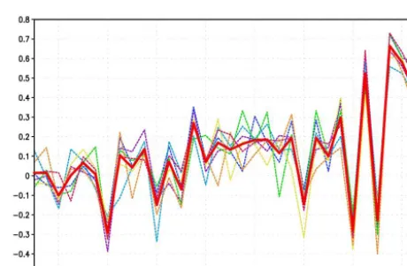
More coherent behavior of model trajectories after year 1980 could be seen for the North Atlantic (45–65◦N) tem-perature (Fig. 5). Indeed, the temtem-perature deviates from its 1850–1899 mean by 1.5 root mean square deviation in the early 2000s. The NA temperature index in the model shows notable oscillations with periods of about 30–40 and 60– 80 years (close to the 25 and 80 years for the observations), and three trajectories have correct strongly positive NA tem-perature anomalies in the 21st century.
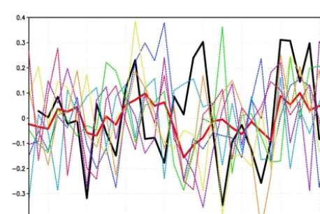
Another important climate feature that could be respon-sible for the changes in the GMST growth rate is the PDO measured by its index defined as the normalized projection of the SST anomaly on a specific pattern in the North Pacific at 20–60◦N. The 5-year average PDO index for observations and model data is presented in Fig. 6. For the observations, one can see maxima at years 1930–1940 and 1980–1995 and
Figure 5.The 5-year mean SST anomaly (K) with respect to 1850– 1899 in the North Atlantic (45–65◦N) for ERSSTv4 data (thick solid black); model mean (thick solid red). Dashed thin lines rep-resent data from individual model runs. Colors correspond to indi-vidual runs as in Fig. 1.
Figure 6.The 5-year mean PDO index (K) for ERSSTv4 data (thick solid black); model mean (thick solid red). Dashed thin lines repre-sent data from individual model runs. Colors correspond to individ-ual runs as in Fig. 1.
a prolonged minimum during 1950–1975. None of the model trajectories reflects observed time series of the PDO index for the same reasons discussed earlier in the paragraph devoted to the AMO. Again the model does not need correct PDO index dynamics to predict GMST behavior.
Figure 7.September Arctic sea ice extent (1012m2) for observa-tions (Comiso and Nishio, 2008) (thick solid black); model mean (thick solid red). Dashed thin lines represent data from individual model runs. Colors correspond to individual runs as in Fig. 1.
one in the observations (reduction from 7–7.5 million km2in the 1980s to 4–5.5 million km2 in the 2000s). In other runs Arctic sea ice loss is underestimated by a factor of 1.5–3, and in one run (green) one can even see some increase in Arctic sea ice area during the last decades. Our results sug-gest that the rapid decrease in Arctic sea ice extent near year 2000 was partially induced by external forcing; however, the role of internal variability can be very important (the range of the sea ice extent year-to-year variability could be estimated as 3.0 million km2).
The stratosphere is more sensitive to global changes than the troposphere. One can see in the observations stratospheric cooling by several degrees during the last decades. In the ERA-Interim reanalysis data (Fig. 8) the global and annual mean temperature at 5 hPa in year 2014 is 3 K lower than in year 1979. All model runs show a gradual decrease in strato-spheric temperature during all periods of the historical run from 1850 to 2014, but the rate of decrease in 1979–2014 is highest and equal to 2.5 K, which is slightly below the ab-solute value observed. This strong decrease is consistent in all model runs and is likely produced by combined effects of CO2increase and ozone decrease. Oscillations of global mean temperature at 5 hPa with a period of 10–12 years rep-resent the prescribed solar cycle.
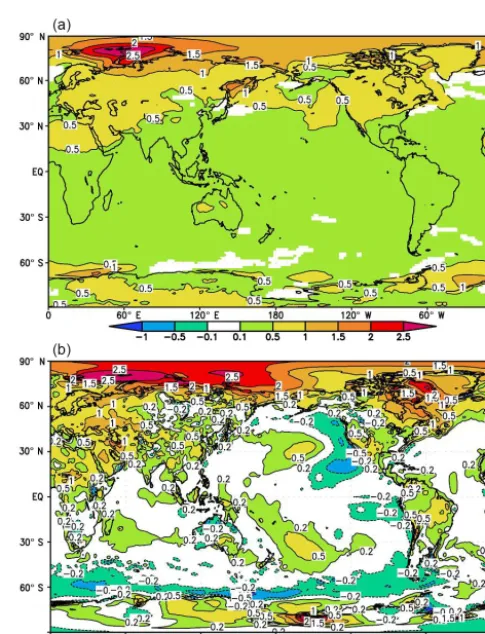
One of the characteristic features of climate changes in recent decades is a specific geographical pattern of surface temperature trends. Figure 9 shows the near-surface air tem-perature difference between 2000–2014 and 1985–1999 ac-cording to ERA-Interim reanalysis and model mean data. Statistical significance for model data was estimated using at test, and the 99 % confidence level was used. Reanaly-sis data look noisier than model mean, but some observed features are reproduced well by the model ensemble.
Maxi-Figure 8.Annual mean global mean temperature (K) at 5 hPa for ERA-Interim data (black) and model data (dashed color lines).
Figure 9.Annual mean near-surface air temperature (K) in 2000– 2014 minus 1985–1999 for model mean data(a); shading represents the 99 % level of significance; ERA-Interim data(b).
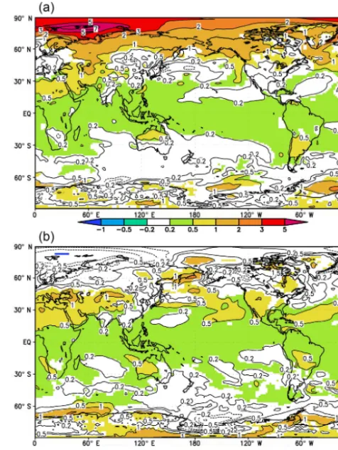
low-data. Otherwise, in the first case (blue) the Arctic warming in some areas is as large as 7 K, and midlatitudinal warm-ing over Eurasia and North America is higher than in model average data.
4 Conclusions
Seven historical runs for 1850–2014 with the climate model INM-CM5 were analyzed. It is shown that the magnitude of the GMST rise in model runs agrees with the estimate based on the observations. All model runs reproduce the stabiliza-tion of GMST in 1950–1970, fast warming in 1980–2000, and a second GMST stabilization in 2000–2014, suggesting that the major factor for predicting GMST evolution is the external forcing rather than system internal variability. Nu-merical experiments with the previous model version (IN-MCM4) for CMIP5 showed unrealistic gradual warming in 1950–2014. The difference between the two model results could be explained by more accurate modeling of the strato-spheric volcanic and tropostrato-spheric anthropogenic aerosol ra-diation effect (stabilization in 1950–1970) due to the new aerosol block in INM-CM5 and more accurate prescription of the TSI scenario (stabilization in 2000–2014) in the CMIP6 protocol. Four of seven INM-CM5 model runs simulate the acceleration of warming in 1920–1940 in a correct way; the other three produce it earlier or later than in reality. This in-dicates that for the warming during 1920–1940 the climate system natural variability plays a significant role.
No model trajectory reproduces the correct time behav-ior of the AMO and PDO indices. Taking into account our results on the GMST modeling one can conclude that an-thropogenic forcing does not produce any significant impact on the dynamics of the AMO and PDO indices, at least for the INM-CM5 model. In turn, the correct prediction of the GMST changes in 1980–2014 and the increase in ocean heat uptake in 1995–2014 does not require correct phases of the AMO and PDO as all model runs have correct values of the GMST, while in at least three model experiments the phases of the AMO and PDO are opposite to the observed ones in that time. The variance explained by PDO and AMO is sim-ilar in the model and in the observations. The North Atlantic
Figure 10.Annual mean near-surface air temperature (K) in 2000– 2014 minus 1985–1999 for the model run with highest(a)and low-est(b)warming in the Arctic. Shading represents the 99 % level of significance.
SST time series produced by the model correlates better with the observations in 1980–2014. Three out of seven trajecto-ries have a strongly positive North Atlantic SST anomaly as in the observations (in the other four cases we see near-to-zero changes for this quantity).
The INM-CM5 has the same skill for prediction of the Arctic sea ice extent in 2000–2014 as CMIP5 models, in-cluding INMCM4. It underestimates the rate of sea ice loss by a factor between 2 and 3. In one extreme case the magni-tude of this decrease is as large as in the observations, while in the other the sea ice extent does not change compared to the preindustrial age. In part this could be explained by the strong internal variability of Arctic sea ice, but obviously the new version of INMCM and the new CMIP6 forcing proto-col do not improve the prediction of the Arctic sea ice extent response to anthropogenic forcing.
warming over the Southern Ocean. Case-to-case variability is very important here as well.
The decrease in stratospheric temperature at 5 hPa during the period of 1979–2014 is successfully reproduced by the model in all experiments. The magnitude of the temperature drop is close to the one for ERA-Interim data (2.5 and 3 K).
Data availability. Data on global mean near-surface
tem-perature HadCRUT4 are available at https://crudata.uea.ac. uk/cru/data/temperature/ (last access: 30 March 2018). The oceanic temperature dataset ERSSTv4 can be downloaded at https://www1.ncdc.noaa.gov/pub/data/cmb/ersst/v4/netcdf/ (last access: 30 March 2018). The ERA-Interim reanalysis can be downloaded at https://www.ecmwf.int/en/forecasts/datasets/ archive-datasets/reanalysis-datasets/era-interim (last access: 30 March 2018). INM-CM5 model output is now available by request to the first author ([email protected]), but will be added to the CMIP6 database.
Author contributions. AG produced model runs and collected
model output; EV performed data processing.
Competing interests. The authors declare that they have no con-flict of interest.
Acknowledgements. The study was performed at the Institute of Numerical Mathematics of the Russian Academy of Sciences and supported by the Russian Science Foundation, grant 14-27-00126. Climate model runs were produced with the supercomputer of the Joint Supercomputer Center of the Russian Academy of Sciences and supercomputer Lomonosov at Moscow State University. Edited by: Christian Franzke
Reviewed by: two anonymous referees
References
Bindoff, N. L., Stott, P. A., AchutaRao, K. M., Allen, M. R., Gillett, N., Gutzler, D., Hansingo, K., Hegerl, G., Hu, Y., Jain, S., Mokhov, I. I., Overland J., Perlwitz, J., Sebbari, R., and Zhang, X.: Detection and Attribution of Climate Change: from Global to Regional, in: Climate Change 2013: The Physical Science Basis. Contribution of Working Group I to the Fifth Assessment Report of the Intergovernmental Panel on Climate Change, edited by: Stocker, T. F., Qin, D., Plattner, G.-K., Tignor, M., Allen, S. K., Boschung, J., Nauels, A., Xia, Y., Bex, V., and Midgley, P. M., Cambridge University Press, Cambridge, United Kingdom and New York, NY, USA, 2013.
Checa-Garcia, R., Shine, K. P., and Hegglin, M. I.: The contri-bution of greenhouse gases to the recent slowdown in global-mean temperature trends, Environ. Res. Lett., 11, 094018, https://doi.org/10.1088/1748-9326/11/9/094018, 2016.
Comiso, J. C. and Nishio, F.: Trends in the sea ice cover using enhanced and compatible AMSR-E, SSM/I, and SMMR data, J. Geophys. Res.-Oceans, 113, C02s07, https://doi.org/10.1029/2007JC004257, 2008.
Dee, D. P., Uppala, S. M., Simmons, A. J., Berrisford, P., Poli, P., Kobayashi, S., Andrae, U., Balmaseda, M. A., Balsamo, G., Bauer, P., Bechtold, P., Beljaars, A. C. M., van de Berg, L., Bid-lot, J., Bormann, N., Delsol, C., Dragani, R., Fuentes, M., Geer, A. J., Haimberger, L., Healy, S. B., Hersbach, H., Holm, E. V., Isaksen, L., Kallberg, P., Kohler, M., Matricardi, M., McNally, A. P., Monge-Sanz, B. M., Morcrette, J. J., Park, B. K., Peubey, C., de Rosnay, P., Tavolato, C., Thepaut, J. N., and Vitart, F.: The ERA-Interim reanalysis: configuration and performance of the data assimilation system, Q. J. Roy. Meteorol. Soc., 137, 553– 597, https://doi.org/10.1002/qj.828, 2011.
Dong, L. and McPhaden, M. J.: The role of external forcing and internal variability in regulating global mean surface tempera-tures on decadal timescales, Environ. Res. Lett., 12, 034011, https://doi.org/10.1175/JCLI-D-17-0138.1, 2017.
Eyring, V., Bony, S., Meehl, G. A., Senior, C. A., Stevens, B., Stouffer, R. J., and Taylor, K. E.: Overview of the Coupled Model Intercomparison Project Phase 6 (CMIP6) experimen-tal design and organization, Geosci. Model Dev., 9, 1937-1958, https://doi.org/10.5194/gmd-9-1937-2016, 2016.
Huang, B., Banzon, V. F., Freeman, E., Lawrimore, J., Liu, W., Pe-terson, T. C., Smith, T. M., Thorne, P. W., Woodruff, S. D., and Zhang, H. M.: Extended Reconstructed Sea Surface Temperature version 4 (ERSST.v4): Part I. Upgrades and intercomparisons, J. Climate, 28, 911–930, 2015.
McCusker, K. E., Fyfe, J. C., and Sigmond, M.: Twenty-five winters of unexpected Eurasian cooling unlikely due to Arctic sea-ice loss, Nat. Geosci., 9, 838–843, 2016.
Meehl, G. A., Arblaster, J. M., Fasullo, J. M., Hu, A., and Tren-berth, K. E.: Model-based evidence of deep-ocean heat uptake during surface-temperature hiatus periods, Nature Clim. Change, 1, 360–364, 2011.
Morice, C. P., Kennedy, J. J., Rayner, N. A., and Jones, P. D.: Quantifying uncertainties in global and regional tem-perature changes using an ensemble of observational esti-mates: the HadCRUT4 dataset, J. Geophys. Res., 117, D08101, https://doi.org/10.1029/2011JD017187, 2011.
Overland, J. E., Wood, K. R., and Wang, M.: Warm Arctic-cold con-tinents: climate impacts of the newly open Arctic Sea, Polar Res., 30, 15787, https://doi.org/10.3402/polar.v30i0.15787, 2011. Rhein, M., Rintoul, S. R., Aoki, S., Campos, E., Chambers, D.,
Feely, R. A., Gulev, S., Johnson, G. C., Josey, S. A., Kostianoy, A., Mauritzen, C., Roemmich, D., Talley, L. D., and Wang, F.: Observations: Ocean, in: Climate Change 2013: The Physical Science Basis. Contribution of Working Group I to the Fifth Assessment Report of the Intergovernmental Panel on Climate Change, edited by: Stocker, T. F., Qin, D., Plattner, G.-K., Tig-nor, M., Allen, S. K., Boschung, J., Nauels, A., Xia, Y., Bex, V., and Midgley, P. M., Cambridge University Press, Cambridge, United Kingdom and New York, NY, USA, 2013.