Some Characterization Results based on Conditional Expectation of function of Dual Generalized Order Statistics

Some Characterization Results Based on Conditional Expectation

of Function of Dual Generalized Order Statistics

M. I. Khan

Department of Statistics & Operations Research Aligarh Muslim University

Aligarh, 202 002. India [email protected] M. Faizan

Department of Statistics & Operations Research Aligarh Muslim University

Aligarh, 202 002. India [email protected]

Abstract

Two families of probability distributions are characterized through the conditional expectations of dual generalized order statistics (dgos) and spacing of two dgos conditioned on a non-adjacent dual generalized order statistics. Further, some of its deductions are also discussed.

Keywords: Characterization, Conditional expectation, Dual generalized order statistics, Probability distributions.

1. Introduction

The concept of generalized order statistics (gos) has been introduced as a unified approach to a variety of models of ordered random variables with different interpretation (Kamps, 1995), such as ordinary order statistics, sequential order statistics, progressive type II censoring, record values and Pfeifer’s records. Generalized order statistics serve as a common approach to a structural similarities and analogies. Several of these models can be effectively applied, e.g., in reliability theory. Using this concept of gos, Burkschatet al. (2003) introduced the concept of dual generalized order statistics (dgos) that enables a common approach to descending ordered random variables like reverse ordered order statistics, lower record values etc.

Let X1,X2,,Xn be a sequence of independent and identically distributed (iid) random variable with absolutely continuous distribution function (df) F(x) and the probability density function (pdf) f (x), x(,). Further, let nN , n2, k 1,

1 1

2

1, , , )

(

~ 

 

 m m m_n n

m  ,





  n 1

r

j j

r m

M , such that _r knrM_r 1, for all

} 1 , , 2 , 1

{ 

 n

r  . Then, X(r,n,m~, k), r 1,2,,n are called dgos if their joint pdf

is given by

) ( )] ( [ ) ( )] (

[ 1

1

1 1

1 n

k n n

i i

m i n

j j F x f x F x f x

k  i 

 

 

   

       

  





 (1.1)

Here we will assume two cases:

Case I: m1 m2 mn1 m.

The pdf of the rth dgos is given by (Burkschatet al., 2003)

1 1

1 )

, , ,

( ( ) ₍ _1)![ ( )]  ( )[ ( ( ))]

rnmk  _r m r

X x _rc F x f x g F x

f r (1.2)

The joint pdf of the rth and sth dgos is

)) ( ( ) ( )] ( [ )! 1 (

)! 1 ( ) ,

( 1 1

) , , , ( ), , , ,

( x y _r c_{s r} F x f x g F x

f r

m m

s k

m n s X k m n r

X   

   

) ( )] ( [ ))] ( ( )) ( (

[h F y h F x s r 1 F y s 1f y

m

m    

  ,   y x, (1.3)

where

   

  

  



 

1 ,

log

1 ,

1 1 )

( 1

m x

m x

m x

h_m m

and

) 1 ( ) ( )

( _{m m}

m x h x h

g   , x[01,).

The conditional pdf of X(s,n,m,k) given X(r,n,m,k) x, 1rsn

 ) | ( | y x f_sr

1 1 )! 1 (srs c_r

c

) ( )]

( [ ) 1 (

)] ( [ ] )) ( ( ))

( [(

1 1

1 1

1 1

y f x

F m

y F y

F x

F

r

s r

s

r s m m



 

 

  

 

 _  (1.4)

Case II: i j i  j,i, j 1,,n1.

The pdf of therth dgos is given by (Burkschatet al., 2003)

) ( ) , ~ , ,

( x

f_X _{rn m k} 1

1

1 ( ) ( )[ ( )] 







_{c f x} r _{a r F x} i

i i

r  (1.5)

and the joint pdf of the rth and sth dgos is

j

x F

y F s a c

y x

f s

r j

r j s

k m n s X k m n r X



     





   

 ( , ) ( ) ₍( ₎)

1 ) ( 1

) , ~ , , ( , ) , ~ , , (

) (

) ( ) (

) ( )] ( [ ) (

1 F y

y f x F

x f x F r a

r

i i

i

    

   





 _(1.6)

where

n r i r

a r _{j i}

i j

j j i

i 



_    



 ( ) , , 1

1 )

(

1

  

 (1.7)

and

n s i r s

a s _{j i}

i j r

j j i r

i 



_     

 

 ( ) , , 1

1 )

(

1 )

( _{ }



Thus, the conditional pdf of X(s,n,m~,k) _{given X}(_r,_n,_m~,_k)_x, 1_r _s_n is

) (

) ( )

( ) ( ) ( )

| (

1

1 ) ( 1

1

| y x _cc a s _FF _xy _Ff _xy

f s i

r i

r i r

s r

s



   



      



, x y (1.9)

If m0, k 1, then X(r,n,m,k) reduces toXnr1:n, the (nr1)thorder statistics, from a sample of size n and when m1, then X(r,n,m,k) _{reduces to the r}th _k lower record value (Pawlas and Szynal, 2001). A number of results on characterization of distributions of dual generalized order statistics are available in the literature. For a detailed survey one may refer to Ahsanullah (2004), Mbah and Ahsanullah (2007), Khan et al. (2009) and Khan et al. (2010) and references contained therein. In this paper, two general classes of distributions

0 , )

(_{x e} ( ) _a

F ah x _{,x(,) (1.10)}

and

c b x h a x

F( )[ ( ) ] , x(,) (1.11)

have been characterized through conditional expectation of function of dgos,where

c b

a, , and h(x) are so chosen that F(x)in (1.10) and (1.11) are df .

It may be noted that the df F(x) and thepdf f(x) in (1.10) and (1.11) are related respectively as

) (

) ( )

(

x h a

x f x

F  _ (1.12)

and

] ) ( [

) ( )

( ) (

b x ah

x h ac x

F x f

 

 (1.13)

Khan et al. (2010) have characterized the general class of distributions through conditional expectation of dgos conditioned on non-adjacent dgos.We have extended the result of Khan et al. (2010) for the difference of the conditional expectations conditioned on non-adjacentdgos, its particular cases for order statistics, lower record statistics as obtained by Khanet al.(2011) and Faizan and Khan (2011) are discussed.

2. Characterizations of distributions when

j i 

  i j,i, j 1,,n1.

Theorem 2.1:Let X be an absolutely continuous random variable with the df F(x) and thepdf f(x) in the interval(,), where  and  may be finite or infinite, then for

n t s r    

1 ,

] ) , ~ , , ( | )} , ~ , , ( { )} , ~ , , ( {

[h X s n m k h X t n m k X l n m k x

E     



 



 s

t

j j

a 1

1 1

if and only if

0 , )

(_{x e} ( ) _a

F ah x _(2.2)

where h(x) is a monotonic and differentiable function of x such that h(x)0 as x 

and h(x)F(x)0 as x.

Proof:First we shall prove that (2.2) implies (2.1). It can be seen (Athar et al., 2008) that ] ) , ~ , , ( | )} , ~ , , 1 ( { )} , ~ , , ( {

[h X t n m k h X t n m k X r n m k x

E      

dy x F y F y h t a c

c t _x i

r i r i r t   _      





    ) ( ) ( ) ( ) ( 1 ) ( 1 2

Therefore, for1rstn

] ) , ~ , , ( | )} , ~ , , ( { )} , ~ , , ( {

[h X s n m k h X t n m k X r n m k x

E     



           1 0 ] ) , ~ , , ( | )} , ~ , ,1 ( { )} , ~ , , ( { [ t s i x k m n r X k m n i s X h k m n i s X h E



         s t j x k m n r X k m n j X h k m n j X h E 1 ] ) , , , ( | )} , , , 1 ( { )} , , , ( { [







              s t j x j r i r i r j _dy x F y F y h j a c c i 1 1 ) ( 1 2 ) ( ) ( ) ( ) (  



    s t j j a ₁ 1 1

 , in view of (1.9) and (1.12)

This proves the necessary part.

For the sufficiency part, we have at



   s t j j a c 1 1 1  )} , ~ , , ( {

[h X t n m k

E  _h{_X(_s,_n,_m~,_k)}|_X(_r,_n,_m~,_k) _x]_c

dy y F y f x F y F y h t a c c i x t r i r i r t ) ( ) ( ) ( ) ( ) ( ) ( 1 ) ( 1 1   _    





    c dy y F y f x F y F y h s a c c i x s r i r i r s _       





    ) ( ) ( ) ( ) ( ) ( ) ( 1 ) ( 1 1   (2.3)

Differentiating (2.3) w.r.t.x we have

) ( ) ( ) ( ) ( ) ( ) ( ) ( 1 ) ( 1 1 1 ) ( 1

1 _{a t}

c c x F x f x h t a c c x F x f t r i r i i r t t r i r i r

t





        _{ } dy x F y f y F y h x i i



     )] ( [ ) ( )] ( [ ) ( 1 ) ( ) ( ) ( ) ( 1 ) ( 1

1 _{a s h x}

c c x F x f s r i r i r s



     0 )] ( [ ) ( )] ( [ ) ( ) ( ) ( ) ( 1 1 ) ( 1 1 _ 





     _dy x F y f y F y h s a c c x F x

f s x

Rearranging the terms in (2.4) and noting that ( ) 0 1

)

( _



 

s a

s

r i

r

i ,

c

r





r1

c

r1 and )

( ) (

)

( ( )

1 )

1

( _{t a t}

a r

i i r r

i      , we get

)] ( )

(

[gt_|r x gt_|r₁ x [gs|r(x)gs|r1(x)]0

where

] ) , ~ , , ( | )} , ~ , , ( { [ ) (

| x E h X s n m k X r n m k x

gsr    

or,

c x g x g x

g x g x g x

gt|r( ) s|r( ) t|r1( ) s|r1( ) t|s( ) s|s( ) (2.5)

Noting thatgs_|s(x)h(x), we have

c x h x

gt|s( ) ( )

i.e.



 

   

 t

s

j j

a x h x k m n s X k m n t X h E

1

1 1 ) ( ] ) , ~ , , ( | )} , ~ , , ( {

[ _ (2.6)

Using the result (Khanet al., 2006)

) ( ] ) , ~ , , ( | )} , ~ , , ( {

[h X t n m k X s n m k x g_| x

E     ts ,

implies



_e x Au du

x

F( ) ( ) (2.7)

where

) ( )]

( ) ( [

) ( )

(

| 1

| 1

| _{ah u}

u g u g

u g u

A

s t s

t s

s

t _{ }

  

 

 (2.8)

we get,

0 , )

(x e ( ) a

F ah x

and hence the Theorem.

Remark 2.1: Atsr, [ { ( , ,~, )}| ( , ,~, ) ] 1 1 ( )

1

x h a

x k m n s X k m n t X h

E t

s

j j

 

 





  

as obtained by Khanet al. (2010).

Remark 2.2: Atm0,k 1, we will get the following result for order statistics for n

t s r   

1

] |

)} {( )} {(

[h X : h X : X : x

E sn  tn rn 





  



 s

t

j n j

a 1 1

1 1

] |

)} {( )} {(

[h X : h X : X: y

E sn  rn tn 









 1 s 1 1

r j j a as obtained by Khanet al.(2011).

Remark 2.3: Atm1, k1 and

a

Corollary 2.1: Under the conditions as given in Theorem 2.1 and for 1rstn )

( )}] , ~ , , ( { )} , ~ , , ( {

[h X s n m k h X r n m k h x

E    

] ) , ~ , , ( | )} , ~ , , ( {

[h X s n m k X r n m k x

E   

 (2.9)

if and only if

0 , )

(_{x e} ( ) _a

F ah x _(2.10)

Proof:The proof from Theorem 2.1 and Remark 2.1.

Further, putting m0,k 1 in equation (2.9), we will get the result for order statistics as follows,

) ( )}] {(

)} {(

[h X : h X : h x

E rn  sn  E[h{(Xr:n)}|Xs:n x]

Theorem 2.2: LetX be an absolutely continuous random variable with the df F(x) and the pdf f(x) in the interval(,), where  and  may be finite or infinite, then for

n t s r   

1 ,

] ) , ~ , , ( | )} , ~ , , ( {

[h X t n m k X l n m k x

E   

1 , , ]

) , ~ , , ( | )} , ~ , , ( {

[ *

| *

|      

a_ts E h X s n m k X l n m k x b_ts l r r (2.11) if and only if

c b x h a x

F( )[ ( ) ] (2.12)

where



  

 t

s

j j

j s

t _c

c a

1 *

| _{1 }



and (1 * )

| *

|s ts

t _ab a

b  

Proof: First we shall prove that (2.12) implies (2.11). In view of Khan et al. (2010), we have

] ) , ~ , , ( | )} , ~ , , ( {

[h X t n m k X r n m k x

E    *

| *

|r ( ) tr t h x b

a 



a b a b x h

atr 

  



 _

 * ( )

| (2.13)

where

* | *

| 1

*

| ₁ sr ts

t

r

j j

j r

t _c a a

c

a 







  



and

) 1

( *

| *

|r tr

t _ab a

b  

] ) , ~ , , ( | )} , ~ , , ( {

[h X t n m k X r n m k x

E   

a b a b x h a

ats sr 

  



 _

 * ( )

| *

|

* | *

| *

|s sr ( ) ts

t a h x _ab _ab b_aa

a _

  

 

    



 _



a b



  



 * [ { ( , ,~, )}| ( , ,~, ) ]

| E h X s n m k X r n m k x

a_ts *

For the sufficiency part, we have dy y F y f x F y F y h t a c c i x t r i r i r t ) ( ) ( ) ( ) ( ) ( ) ( 1 ) ( 1 1   _    





    i x F y F y h s a c c

a s x

r i r i r s s t   _     





    ) ( ) ( ) ( ) ( 1 ) ( 1 1 *

| _Ff(₍y_y)₎ dybt*|s (2.14)

Differentiating (2.14) w.r.t.x and rearranging, we get

) ( ) ( ) ( 1 ) ( 1 1 1 ) ( 1

1 _{a t}

c c x h t a c c t r i r i i r t t r i r i r

t





        _    _   



 dy

x F y f y F y h x i i    )] ( [ ) ( )] ( [ ) ( 1 ) ( ) ( ) ( 1 ) ( 1 1 1 ) ( 1 1 *

| _cc a s h x _cc a s

a s r i r i i r s s r i r i r s s

t





        _        





 dy

x F y f y F y h x i i    )] ( [ ) ( )] ( [ ) ( 1

After noting that ( ) 0 1 ) ( _



  s a s r i r

i ,cr r1cr1and ai(r1)(t)(r1i)ai(r)(t), we get

) ( 1 ) ( 1 1

1 _{a t}

c c t r i r i r t r



      dy x F y f y F y h x i i



   )] ( [ ) ( )] ( [ ) ( 1 ) ( 2 ) 1 ( 1

1 _{a t}

c c t r i r i r t r



    

  dy

x F y f y F y h x i i



   )] ( [ ) ( )] ( [ ) ( 1    



     _{( )} 1 ) ( 1 1 1 *

| _c c a s

a s r i r i r s r s t  dy x F y f y F y h x i i



   )] ( [ ) ( )] ( [ ) ( 1 ) ( 2 ) 1 ( 1

1 _{a s}

c c s r i r i r s r



       _  



 dy

x F y f y F y h x i i    )] ( [ ) ( )] ( [ ) ( 1 That is, )] ( ) (

[ | | 1

1 gtr x gtr x

r  

 at*|sr1[gs|r(x)gs|r1(x)] where ] ) , ~ , , ( | )} , ~ , , ( { [ ) (

| x E h X s n m k X r n m k x

gsr    

or, ) ( ) ( ) ( )

( *| | | 1 *| | 1

| x a g x g x a g x

gtr  ts sr  tr  ts sr

* | |

* |

|s( ) ts ss( ) ts

t x a g x b

g  



_{ (2.15)}

Noting thatgs_|s(x)h(x), we have *

| *

|

|s( ) ts ( ) ts t x a h x b

g  

i.e. * | * | ( ) ] ) , ~ , , ( | )} , ~ , , ( {

[h X t n m k X s n m k x atsh x bts

Using the result (Khanet al., 2006)

) ( ] ) , ~ , , ( | )} , ~ , , ( {

[h X t n m k X s n m k x g_| x

E     ts ,

implies

  



x Au du e

x

F( ) ( ) (2.17)

We get

c b x h a x

F( )[ ( ) ] and hence the Theorem.

Remark 2.4:It may be seen that when _i  _{j but} m_i m_j m_{, then}

)! ( )! 1 (

1 )

1 ( )

1 (

1 )

( ₁

) (

i t r i m

t

a_ir _{t r} t i

   



 _{ } 

)! ( )! 1 (

1 )

1 ( ) 1 (

1 )

( ₁

i r i

m r

a_{i r} r i

 

 

 _ 

and consequently (1.5) will reduce to (1.2), (1.6) to (1.3).

Remark 2.5:Atm0,k 1, we will get result for order statistics as follows, ]

) ( | )} {(

[h X : X : x

E tn rn 

* | :

: *

|s [ {( sn)}|( rn) ] ts

t E h X X x b

a    

 or

] ) ( | )} {(

[h X : X : y

E rn tn  ar*|s E[h{(Xs:n)}|(Xt:n) y]br*|s where





 

 1 *

| ₁

s

r j s

r c_cj _j

a and (1 * )

| *

|s rs

r _ab a

b  

as obtained by Khanet al.(2011).

Remark 2.6:Ats r, it reduces to as obtained by Khanet al. (2010).

Remark 2.7: At

c a

a , b1 and c then _{F(x)[ah(x)b]}c _eah(x) _as

obtained in Theorem 2.1.

3. Conclusion

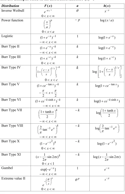
In this paper, conditional expectation of the difference of two dgos conditioned on non-adjacent dgos are considered to characterize the df _F(x)eah(x) _{whose particular}

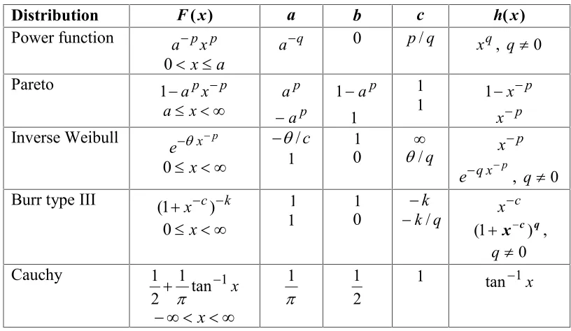
cases are given in the Table 2.1 with proper choice ofa,b, candh(x). Also c

b x ah x

F( )[ ( ) ] is characterized through the conditional expectation of dgos

Table 2.1: Examples based on the distribution functionF(x)eah(x)

Distribution F(x) a h(x)

Inverse Weibull _x p e_ 

  x 0

 _xp

Power function p

a x

     

a x  0

p

 _log(x/a)

Logistic _(1ex₎1

   

 x

1 _log(1ex₎

Burr Type II _(1ex₎k    

 x

k _log(1ex₎

Burr Type III _(1xc₎k    x 0

k _log(1xc₎

Burr Type IV _c k

x x

c 

    

  

      

 1/

1

c x  0

k

    

  

      

 c

x x c 1/ 1

log

Burr Type V _(1cetanx₎k

2 2



 _{ }

 x

k _log(1cetanx₎

Burr Type VI _(1ceksinhx₎k    

 x

k _log(1ceksinhx₎

Burr Type VII _x k

   

  

2 tanh 1

   

 x

k



   

  

2 tanh 1

log x

Burr Type VIII k

x e 

  



2_tan1



   

 x

k



   



2_tan1_ex log



Burr Type X _{e x k}

) 1

(   2   x 0

k



) 1

(

log ex2

Burr Type XI _{x sin2 x)k} 2

1

( 





1 0x

k



) 2 sin 2

1 (

log x x





Gumbel _exp[ex_]    

 x

1 _ex

Extreme value II p

x e 

     

  x 0

p

Table 2.2: Examples based on the distribution functionF(x)[ah(x)b]c

Distribution F(x) a b c h(x)

Power function _ap_xp

a x  0

q

a 0 p/q xq, q 0

Pareto _1ap_xp   x a

p

a

p

a



p

a

 1

1

1

1 x p

  1

p

x

Inverse Weibull _x p

e 

   x 0

c /

 

1 10 /q x_pp

x q

e  , q 0 Burr type III _(1xc₎k

   x 0

1

1 10 kk/q x c



q c

x )

1

( _  _,

0 

q

Cauchy 1 _{tan 1x}

2

1_ 



   

 x 

1

2

1 1 _tan1_x

Acknowledgement

The authors are grateful to Professor A.H. Khan, Department of Statistics and Operations Research, Aligarh Muslim University for his valuable suggestions in preparing this paper. We are also thankful to the referees for their useful suggestions, which lead to the improvement of the manuscript.

References

1. Ahsanullah, M. (2004). A characterization of the uniform distribution by dual generalized order statistics.Comm. Statist. Theory Methods, 33, 2921-2928. 2. Athar Haseeb, Anwar, Z. and Khan, R.U. (2008). On recurrence relations for the

expectations of function of lower generalized order statistics. Pakistan. J. Statist., 24, 111-122.

3. Burkschat, M., Cramer, E. and Kamps, U. (2003). Dual generalized order statistics.Metron, LXI (1), 13-26.

4. Faizan, M. and Khan, M.I. (2011). A characterization of continuous distributions through lower record statistics.Prob Stat Forum., 4, 39-43.

5. Kamps, U. (1995). A Concept of Generalized Order Statistics, B.G. Teubner Stuttgart.

6. Khan, A.H., Anwar, Z. and Chishti, S. (2010). Characterization of continuous distributions through conditional expectation of functions of dual generalized order statistics.Pakistan J. Statist., 26, 615-628.

8. Khan, A.H., Faizan, M. and Haque, Z. (2011). Characterization of continuous distributions via conditional expectations of non-adjacent order statistics. Submitted for publication.

9. Khan, M.J.S., Haque, Z. and Faizan, M. (2009). On characterization of continuous distributions conditioned on a pair of non-adjacent dual generalized order statistics.Aligarh J. Statist., 29,107-119.

10. Mbah, A.K. and. Ahsanullah, M. (2007). Some characterization of the power function distribution based on lower generalized order statistics. Pakistan J. Statist., 23, 139-146.