Statistics Publications Statistics
2019
Nearest Neighbor Imputation for General
Parameter Estimation in Survey Sampling
Shu Yang
North Carolina State University
Jae Kwang Kim
Iowa State University, [email protected]
Follow this and additional works at:https://lib.dr.iastate.edu/stat_las_pubs
Part of theDesign of Experiments and Sample Surveys Commons, and theStatistical Methodology Commons
The complete bibliographic information for this item can be found athttps://lib.dr.iastate.edu/ stat_las_pubs/261. For information on how to cite this item, please visithttp://lib.dr.iastate.edu/ howtocite.html.
This Book Chapter is brought to you for free and open access by the Statistics at Iowa State University Digital Repository. It has been accepted for inclusion in Statistics Publications by an authorized administrator of Iowa State University Digital Repository. For more information, please contact
Nearest Neighbor Imputation for General Parameter Estimation in Survey
Sampling
Abstract
Nearest neighbor imputation has a long tradition for handling item nonresponse in survey sampling. In this article, we study the asymptotic properties of the nearest neighbor imputation estimator for general
population parameters, including population means, proportions and quantiles. For variance estimation, we propose novel replication variance estimation, which is asymptotically valid and straightforward to
implement. The main idea is to construct replicates of the estimator directly based on its asymptotically linear terms, instead of individual records of variables. The simulation results show that nearest neighbor imputation and the proposed variance estimation provide valid inferences for general population parameters.
Keywords
Bahadur representation, Bootstrap, Jackknife variance estimation, Matching, Missing at random, Quantile estimation
Disciplines
Design of Experiments and Sample Surveys | Statistical Methodology Comments
This is a manuscript of a chapter from Yang, S. and Kim, J. (2019), "Nearest Neighbor Imputation for General Parameter Estimation in Survey Sampling", The Econometrics of Complex Survey Data (Advances in Econometrics, Vol. 39), Emerald Publishing Limited, pp. 209-234. doi:10.1108/
arXiv:1707.00974v1 [stat.ME] 30 Jun 2017
Nearest neighbor imputation for
general parameter estimation in
survey sampling
Shu Yang
∗Jae Kwang Kim
†Abstract
Nearest neighbor imputation is popular for handling item nonre-sponse in survey sampling. In this article, we study the asymptotic properties of the nearest neighbor imputation estimator for general population parameters, including population means, proportions and quantiles. For variance estimation, the conventional bootstrap infer-ence for matching estimators with fixed number of matches has been shown to be invalid due to the nonsmoothness nature of the matching estimator. We propose asymptotically valid replication variance esti-mation. The key strategy is to construct replicates of the estimator directly based on linear terms, instead of individual records of vari-ables. A simulation study confirms that the new procedure provides valid variance estimation.
Key Words: Bahadur representation; Bootstrap; Hot deck; Jackknife vari-ance estimation; Missing at random; Quantile estimation.
∗Department of Statistics, North Carolina State University, North Carolina 27695,
U.S.A.
1
Introduction
Nearest neighbor imputation is popular for handling item nonresponse in survey sampling. In nearest neighbor imputation, the vector of the auxiliary variables is directly used in determining the nearest neighbor. The near-est neighbor is then used as a donor for hot deck imputation. Although these imputation methods have a long history of application, there are rela-tively few papers on investigating their asymptotic properties. Sande (1979) discussed nearest neighbor rules in statistical estimation with hot-deck tation. Lee and S¨arndal (1994) studied methods of nearest neighbor impu-tation. Chen and Shao (2000, 2001) have developed a nice set of asymptotic theories for the nearest neighbor imputation estimator. Abadie and Imbens (2006) studied the matching estimator to estimate the average treatment effect from observational studies. Shao and Wang (2008) proposed methods for constructing confidence intervals for population means and quantiles with nearest neighbor imputation. Kim et al. (2011) presented an application of nearest neighbor imputation for the US Census long form data. However, most of these studies discussed either with a 1-dimensional covariate or only for mean estimation, which is restrictive both theoretically and practically.
Survey statisticians are often interested in various finite population
quan-tities, such as the population means, proportions and quantiles (Francisco and Fuller; 1991; Wu and Sitter; 2001; Berger and Skinner; 2003), to name a few. Some
corresponding sample estimators should be treated differently than others. For example, estimators of population quantiles involve nondifferentiable functions of estimated quantities. Moreover, there often are more than one auxiliary covariates available to facilitate nearest neighbor imputation. The
current framework of nearest neighbor imputation can not cover inferences in these settings.
In this article, we provide a framework of nearest neighbor imputation for general parameter estimation in survey sampling. In general, the match-ing estimators are not root-n consistent (Abadie and Imbens; 2006), where
n is the sample size. Based on a scalar matching variable m summarizing all auxiliary information, we show that nearest neighbor imputation can pro-vide consistent estimators for a fairly general class of parameters. If the matching variable is chosen to be the mean function of the study variable, our method resembles prediction mean matching imputation. However, the validity of predictive mean matching requires the mean function to be cor-rectly specified. Here, we show that the consistency of the nearest neighbor imputation estimator only requires the matching variable to satisfy certain Lipschitz continuity condition. For inference, intrinsically the nearest neigh-bor imputation estimator with fixed number of matches is not smooth. The lack of smoothness makes the conventional replication methods invalid for variance estimation, mainly because the naive replication method distorts the distribution of the number of times each unit is used as a match. We propose new replication variance estimation. Based on the linear representa-tion of the nearest neighbor imputarepresenta-tion estimator, we construct replicates of the estimator directly based on its linear terms. In this way, the distribution of the number of times each unit is used as a match can be preserved, which leads to a valid variance estimation. Furthermore, our replication variance method is flexible, which can accommodate bootstrap and jackknife, among others.
2
Basic Setup
LetFN ={(xi, yi, δi) :i= 1, . . . , N}denote a finite population, wherexi is a
p-dimensional vector of covariates, which is always observed, yi has missing
values, and δi is the response indicator of yi, i.e., δi = 1 if yi is observed and
0 if it is missing. The δi’s are defined throughout the finite population, as in
Fay (1992), Shao and Steel (1999), and Kim et al. (2006). We assume that
FN is a random sample from a superpopulation model ζ, and N is known.
Our objective is to estimate the finite population parameter defined through
µg =N−1PiN=1g(yi) for some knowng(·), orξN = inf{ξ :SN(ξ)≥0}, where
SN(ξ) = N−1PNi=1s(yi −ξ) and s(·) is a univariate real function. These
parameters are fairly general, which cover many parameters of interest in survey sampling. For example, let g(y) = y, µg is the population mean of y,
N−1PN
i=1yi. Let g(y) = I(y < c) for some constant c, µg is the population
proportion ofyless thanc,N−1PN
i=1I(yi < c). Lets(yi−ξ) =I(yi ≤ξ)−α, ξN is the population αth quantile.
LetAdenote an index set of the sample selected by a probability sampling design. Let Ii be the sampling indicator function, i.e., Ii = 1 if unit i is
selected into the sample, and Ii = 0 otherwise. Suppose that πi, the
first-order inclusion probability of unit i, is positive and known throughout the sample. Ifyiwere fully observed throughout the sample, the sample estimator
of µg and ξN are ˆµg = N−1Pi∈Aπ
−1
i g(yi) and ˆξ = inf{ξ : ˆSN(ξ) ≥ 0} with
ˆ
SN(ξ) =N−1Pi∈Aπ
−1
i s(yi−ξ), respectively.
We make the following assumption for the missing data process.
process satisfies pr(δ = 1 | x, y) = pr(δ = 1 | x), which is denoted by p(x), and with probability 1, p(x)> ǫ for a constant ǫ >0.
Our primary focus will be on the imputation estimators ofµgandξN given
by ˆµg,I = N−1Pi∈Aπ −1 i {δig(yi) + (1−δi)g(yi∗)} and ˆξI = inf{ξ : ˆSI(ξ) ≥ 0}, with ˆSI(ξ) = ˆN−1Pi∈Aπ −1 i s(yi − ξ){δis(yi−ξ) + (1−δi)s(yi∗−ξ)}, where y∗
i is an imputed value of yi for unit i with δi = 0. To find suitable
imputed values, the classical nearest neighbor imputation can be described in the following steps:
Step 1. For each unit i with δi = 0, find the nearest neighbor from the
respondents with the minimum distance between xj and xi. Let i(1)
be the index set of its nearest neighbor, which satisfies d(xi(1), xi) ≤
d(xj, xi),for j ∈ AR, where d(xi, xj) is a distance function between xi
and xj. For example, d(xi, xj) = ||xi −xj||, where ||x|| = (xTx)1/2.
Other norms of the form ||x||D = (xTDx)1/2, where D is a positive
definite symmetric matrix D, are equivalent to the Euclidean norm,
since ||x||D ={(Qx)T(Qx)}1/2 =||Qx|| with QTQ =D. In particular,
Mahalanobis distance is commonly used, where D = ˆΣ−1 with ˆΣ the
empirical covariance matrix of x.
Step 2. The nearest neighbor imputation estimators ofµg and ξN are
com-puted by ˆ µg,NNI= 1 N X i∈A 1 πi δig(yi) + (1−δi)g(yi(1)) , (1)
and ˆξNNI= inf{ξ : ˆSNNI(ξ)≥0}, respectively, with
ˆ SNNI(ξ) = 1 N X i∈A π−1 i δis(yi−ξ) + (1−δi)s(yi(1)−ξ) . (2)
In (1) and (2), the imputed values are real observations.
3
Main result
For asymptotic inference, we follow the framework of Isaki and Fuller (1982) where the asymptotic properties of estimators are established under a fixed sequence of populations and a corresponding sequence of random samples. Denote Ep(·) and varp(·) to be the expectation and the variance under the
sampling design, respectively. We impose the following regularity conditions on the sampling design.
Assumption 2 (i) There exist positive constants C1 and C2 such thatC1 ≤ πiNn−1 ≤ C2, for i = 1, . . . , N; (ii) the sequence of the Hotvitz-Thompson
estimators µˆg,HT = N−1Pi∈Aπ
−1
i g(yi) satisfies varp(ˆµg,HT) = O(n−1) and
{varp(ˆµg,HT)}−1/2(ˆµg,HT−µg)| FN → N(0,1) in distribution, as n→ ∞.
Assumption 2 is a widely accepted assumption in survey sampling (Fuller; 2009).
We introduce additional notation. LetA=AR∪AM, where AR and AM
are the sets of respondents and nonrespondents, respectively. Define dij = 1
if yj(1) = yi, i.e., unit i is used as a donor for unit j ∈ AM, and dij = 0
otherwise. We write ˆµg,NNI in (1) as
ˆ µg,NNI= 1 N ( X i∈A 1 πi δig(yi) + X j∈A 1−δj πj X i∈A δidijg(yi) ) = 1 N X i∈A δi πi (1+ki)g(yi), (3) with ki = X j∈A πi πj (1−δj)dij. (4)
Under simple random sampling,ki =Pj∈A(1−δj)dij is the number of times
that unit i is used as the nearest neighbor for nonrespondents.
To study the asymptotic properties of the nearest neighbor imputation estimator ˆµg,NNI, we use the following decomposition:
n1/2(ˆµg,NNI−µg) =DN +BN, (5) where DN =n1/2 " 1 N X i∈A 1 πi {µg(xi) +δi(1 +ki){g(yi)−µg(xi)} −µg # , (6) and BN = n1/2 N X i∈A 1 πi (1−δi){µg(xi(1))−µg(xi)}. (7)
The difference µg(xi(1))−µg(xi) accounts for the matching discrepancy, and
BN contributes to the asymptotic bias of the matching estimator. In general,
if x is p-dimensional, Abadie and Imbens (2006) showed that d(xi(1), xi) =
Op(n−1/p). Therefore, for nearest neighbor imputation with p ≥ 2, the bias
BN =Op(n1/2−1/p)6=op(1) is not negligible.
To address for the matching discrepancy due to a non-scalar x, we first summarize the covariate information into a scalar matching variable m =
m(x), and then apply nearest neighbor imputation based on this scalar vari-able. For simplicity of notation, we may suppress the dependence of m on
x if there is no ambiguity. For nearest neighbor imputation with a scalar matching variable, we then have p = 1 and BN = Op(n−1/2) = op(1). We
assume the superpopulation model and the matching variable m satisfy the following assumption.
Assumption 3 (i) The matching variablem has a compact and convex sup-port, with density bounded and bounded away from zero. Letf1(m)andf0(m)
be the conditional density of m givenδ = 1 and δ= 0, respectively. Suppose that there exist constants C1L and C1U such that C1L≤f1(m)/f0(m)≤C1U;
(ii) µg(x) = E{g(y) | x} and µs(ξ, x) = E{s(y−ξ) | x} sastisfy certain
Lipschitz continuous condition; i.e., there exists a constant C2 such that
|µg(xi)−µg(xj)| < C2|mi −mj| and |µs(ξ, xi)−µs(ξ, xj)| < C2|mi −mj|
for any i and j; (iii) there exists δ > 0 such that E(|g(y)|2+δ | x) and
E(|s(y−ξ)|2+δ |x) are uniformly bounded for any x and ξ in the
neighbor-hood of ξN.
Assumption 3 (i) a convenient regularity condition (Abadie and Imbens; 2006). Assumption 3 (ii) imposes a smoothness condition for µg(x), µs(ξ, x)
andm(x), which is not restrictive (Chen and Shao; 2000). Assumption 3 (iii) is a moment condition for establishing the central limit theorem.
We establish the asymptotic distribution of ˆµg,NNI, with the proof deferred
to the Appendix.
Theorem 1 Under Assumptions 1–2, suppose thatµg(x) =E{g(y)|x}and
σ2
g(x) = var{g(y)| x}. Then, n1/2{µˆg,NNI−µg} → N(0, Vg) in distribution,
as n→ ∞, where Vg =Vgµ+Vge (8) withVµ g = limn→∞nN −2 E[varp{Pi∈Aπ −1 i µg(xi)}], Vge= limn→∞nN −2 E[P i∈A{π −1 i δi(1+ ki)−1}2σg2(xi)], and ki is defined in (4).
We now establish a similar result for ˆξNNI, with the proof deferred to the
Theorem 2 Under Assumptions 1–2, suppose the population parameter ξN
and the population estimating function SN(·) satisfy certain regularity
con-ditions specified in Assumptions A4 and A5. We obtain an asymptotic lin-earization representation of ξˆNNI:
n1/2( ˆξNNI−ξ) = −n1/2{SˆNNI(ξ)−SN(ξ)}/S′(ξ) +op(1). (9)
It follows that n1/2( ˆξ
NNI−ξN)→ N(0, Vξ) in distribution, as n→ ∞, where
Vξ= ˙S(ξN)−2var{SˆNNI(ξN)}, S˙(ξN) = dS(ξN)/dξ, and
var{SˆNNI(ξN)}= lim
n→∞ n N2E varp " X i∈A E{s(yi−ξN)|xi} πi #! +plim n N2 N X i=1 Ii πi δi(1 +ki)−1 2 var [s(yi−ξN)−E{s(yi−ξN)|xi} |xi], (10) and ki is defined in (4).
For illustration, we use quantile estimation as an example.
Example 1 (Quantile estimation) The estimating function for the αth quantile is s(yi−ξ) =I(yi≤ξ)−α, and the population estimating equation
Sα,N(ξ) = FN(ξ)− α, where FN(ξ) = N−1PNi=1I(yi ≤ ξ). The nearest
neighbor imputation estimator ξˆα,NNI is defined as
ˆ
ξα,NNI= inf{ξ : ˆSα,NNI(ξ)≥0},
where Sˆα,NNI(ξ) = ˆFNNI(ξ)−α, FˆNNI(ξ) = ˆN−1Pi∈Aπ
−1 i δi(1 +ki)I(yi ≤ξ), ˆ N = P i∈Aπ −1
i , and ki is defined in (4). Let F(ξ) = pr(y ≤ ξ) be the
forF(ξ), which is asymptotically equivalent to the one usingN instead of Nˆ. Even with a known N, it is necessary to use Nˆ because FˆNNI(ξ) for ξ = ∞
should be 1. The limiting function of Sα,N(ξ) is Sα(ξ) = F(ξ)−α. The
asymptotic linearization representation of ξˆα,NNI is
ˆ ξα,NNI−ξ=− ˆ FNNI(ξ)−FN(ξ) f(ξ) +op(n −1/2), (11) where f(ξ) = F′
(ξ). Expression (11) is called the Bahadur-type representa-tion for ξˆα,NNI (Francisco and Fuller; 1991).
Remark 1 (The choice of the scalar matching variable) By judicious choice, the scalar matching variable should ensure that Assumption 3 holds. If the conditional mean function of the outcome variable given the covariates is feasible, we can choose the matching variable to be the conditional mean function. We note that in this case the proposed nearest neighbor imputa-tion resembles predictive mean matching imputaimputa-tion. However, our method is more general than predictive mean matching imputation, because the latter requires the mean function to be correctly specified.
4
Replication variance estimation
We consider replication variance estimation (Rust and Rao; 1996; Wolter; 2007) for nearest neighbor imputation.
Let ˆµg be the Horvitz-Thompson estimator ofµg.The replication variance
estimator of ˆµg takes the form of
ˆ Vrep(ˆµg) = L X k=1 ck(ˆµ(gk)−µˆg)2, (12)
whereLis the number of replicates,ckis thekth replication factor, and ˆµ(gk)is
the kth replicate of ˆµg. When ˆµg =Pi∈Aωig(yi), we can write the replicate
of ˆµg as ˆµ(gk) =Pi∈Aω
(k)
i g(yi) with some ω(ik) for i∈A. The replications are
constructed such that Ep{Vˆrep(ˆµg)}= varp(ˆµg){1 +o(1)}.
We propose a new replication variance estimation for ˆµg,NNI. Let ωi =
N−1π−1
i . Write ˆµg,NNI−µg = (ˆµg,PMM−ψˆHT) + ( ˆψHT−µψ) + (µψ−µg),where
ˆ
ψHT=Pi∈Aωiψi,ψi =µg(xi)+δi(1+ki){g(yi)−µg(xi)},µψ =N−1PNi=1ψi.
Because µg,NNI−ψˆHT =op(n−1/2) by Theorem 1 and µψ−µg =Op(N−1/2),
we have ˆµg,NNI−µg = ˆψHT−µψ +op(n−1/2), if nN−1 = o(1). Therefore,
with negligible sampling fractions, it is sufficient to estimate the variance of ˆψHT −µψ. Because E( ˆψHT−µψ | FN) = 0, we have var( ˆψHT−µψ) =
E{var( ˆψHT−µψ | FN)}, which is essentially the sampling variance of ˆψHT.
This suggests that we can treat {ψi : i ∈ A} as pseudo observations in
applying replication variance estimator. Otsu and Rai (2016) used a similar idea to develop a wild bootstrap technique for a matching estimator. To be specific, we construct replicates of ˆψHT as follows: ˆψ(HTk) =
P
i∈Aω
(k)
i ψi,where
ωi(k) is the replication weight that account for complex sampling design. The replication variance estimator of ˆψHT is obtained by applying ˆVrep(·) in (12)
for the above replicates ˆψ(HTk). It follows that E{Vˆrep( ˆψHT)} = var( ˆψHT − µψ){1 +o(1)} = var(ˆµg,NNI−µg){1 +o(1)}. Because µg(x) is unknown, we
use a plug-in kernel estimator ˆµg(x).
In summary, the new replication variance estimation for ˆµg,NNI proceeds
as follows:
Step 2. Construct replicates of ˆµg,NNI as
ˆ
µ(g,kNNI) = X
i∈A
ωi(k)[ˆµg(xi) +δi(1 +ki){g(yi)−µˆg(xi)}], (13)
where ωi(k) is the kth replication weight for uniti.
Step 3. Apply ˆVrep(·) in (12) for the above replicates to obtain the replication
variance estimator of ˆµg,NNI.
We now consider a replication variance estimation for ˆξNNI. Following the
previous section, we directly obtain the asymptotic variance of ˆξNNI using
var{SˆNNI(ξ)} and S′(ξ). First to estimate var{SˆNNI(ξ)}, we can use the
similar replication variance estimation earlier in this section. Now to estimate S′
(ξ), we follow the kernel-based derivative estimation of Deville (1999):
ˆ S′(ξ) = 1 Nh X i∈A 1 πi ˆ s(yi−x)K ′ ξ−x h dx (14)
where K(·) is a kernel function in R, K′
(x) = dK(x)/dx, and h is the
bandwidth. Under Assumption A6 for the kernel function and bandwidth and
previously stated regularity conditions on the superpopulations and sampling designs, the kernel-based estimator (14) is consistent for S′
(ξ).
In summary, the new replication variance estimation for ˆξNNIproceeds as
follows:
Step 1. Obtain a consistent kernel estimator ˆµs( ˆξNNI, x)
Step 2. Construct replicates of ˆSNNI( ˆξNNI) as
ˆ
SNNI(k) ( ˆξNNI) = X
i∈A
ωi(k)[ˆµs( ˆξNNI, xi)+δi(1+ki){s(yi−ξˆNNI)−µˆs( ˆξNNI, xi)}].
Step 3. Apply ˆVrep(·) in (12) for the above replicates to obtain the replication
variance estimator of ˆSNNI( ˆξNNI), denoted as Vˆrep{SˆNNI( ˆξNNI)}.
Step 4. Obtain the kernel-based derivative estimator ˆS′
( ˆξNNI), where ˆS′(ξ)
is defined in (14).
Step 5. Calculate the variance estimator of ˆξNNIas ˆS′( ˆξNNI)−2Vˆrep{SˆNNI( ˆξNNI)}.
For illustration, we continue with Example 1.
Example 2 (Quantile estimation (Cont.)) Obtain kernel-based estima-tors for F(ξ) = pr(y ≤ ξ) and f(ξ), denoted as Fˆ(ξ) and fˆ(ξ), respectively. Construct replicates of FˆNNI( ˆξα,NNI) as FˆNNI(k)( ˆξα,NNI) =Pi∈Aω
(k)
i [ ˆF( ˆξα,NNI) +
δi(1 +ki){I(yi ≤ ξˆα,NNI)−Fˆ( ˆξα,NNI)}]. Apply Vˆrep(·) in (12) for the above replicates to obtain the replication variance estimator of FˆNNI( ˆξα,NNI), de-noted as Vˆrep{FˆNNI( ˆξα,NNI)}. Calculate the variance estimator of ξˆα,NNI as
ˆ
f( ˆξα,NNI)−2Vˆrep{FˆNNI( ˆξα,NNI)}.
Theorem 3 Under the assumptions in Theorem 2, suppose that Vˆrep(ˆµg)
in (12) is consistent for varp(ˆµg). Then, if nN−1 = o(1), the replication
variance estimators for µˆg,NNI is consistent, i.e., nVˆrep{µˆg,NNI}/Vg → 1 in
probability, as n → ∞, whereVˆrep(·) is given in (12), the replicates of µˆg,NNI
are given in (13), and Vg is given in (8).
Given that the kernel-based estimatorSˆ′
(ξ)in (14) is consistent forS′
(ξ), the replication variance estimators forξˆNNIis consistent, i.e.,nVˆrep{ξˆNNI}/Vξ→
1 in probability, as n → ∞, where Vˆrep(·) is given in (12), the replicates of
ˆ
SNNI(k) ( ˆξNNI) are given in (15), and Vξ is given in (10).
The formal proof follows by straightforward asymptotic bounding argu-ments from the assumptions and therefore is omitted.
5
Simulation study
In this simulation study, we investigate the performance of the proposed replication variance estimation. For generating finite populations of size
N = 50,000: first, let x1i, x2i and x3i be generated independently from
Uniform[0,1], and x4i, x5i and x6i and ei be generated independently from
N(0,1); then, let yi be generated as (P1) yi = −1 +x1i +x2i +ei, (P2)
yi =−1.5 +x1i+x2i+x3i+x4i+ei, (P3)yi =−1.5 +x1i+· · ·+x6i+ei, (P4)
yi =−1 +x1i+x2i+x21i+x22i−2/3 +ei, (P5)yi =−1.5 +x1i+x2i+x3i+x4i+
x2
1i+x22i−2/3 +ei and (P6) yi =−1.5 +x1i+· · ·+x6i+x21i+x22i−2/3 +ei.
The covariates are fully observed, but yi is not. The response indicator of
yi, δi, is generated from Bernoulli(pi) with logit{p(xi)} = xTi1, where xi
in-cludes all corresponding covariates under each data generating mechanism and 1 is a vector of 1 with a compatible length. This results in the average response rate about 75%. The parameters of interest are µ =N−1PN
i=1yi,
η = N−1PN
i=1I(yi < c), where c is the 80th quantile such that the true
value of η is 0.8, and the median ξ. To generate samples, we consider two sampling designs: (S1) simple random sampling with n = 800; (S2) proba-bility proportional to size sampling. In (S2), for each unit in the population, we generate a size variable si as log(|yi+νi|+ 4), where νi ∼ N(0,1). The
selection probability is specified as πi = 400si/PNi=1si. Therefore, (S2) is
informative, where units with larger yi values have larger probabilities to be
selected into the sample.
For nearest neighbor imputation, the matching scalar variablem is set to be the conditional mean function of ygivenx,m(x), approximated by power series estimation. For investigating the effect of the matching variable, we
consider the power series including all first and second order terms under (P1)–(P3) and only first order terms under (P4)–(P6), so thatm(x) is accu-rate for the mean function under (P1)–(P3) but inaccuaccu-rate under (P4)–(P6). We construct 95% confidence intervals using (ˆµI−z0.975VˆI1/2,µˆI+z0.975VˆI1/2),
where ˆµI is the joint estimate and ˆVI is the variance estimate obtained by
the proposed jackknife variance estimation and a naive jackknife variance estimation that calculates a sample estimator for each replicate. For the jackknife replication method under (S2), in the kth replicate, the replication weights are ωi∗(k)=nωi/(n−1) for all i6=k, and ω
∗(k)
k = 0. In the proposed
jackknife variance estimation, the kth replicates of ˆµNNI, ˆηNNI and ˆξNNI are
given by ˆ µ(NNIk) = n X i=1 ωi(k)[ˆµ(xi) +δi(1 +ki){I(yi < c)−µˆ(xi)}], ˆ η(NNIk) = n X i=1 ω(ik)[ˆµη(xi) +δi(1 +ki){I(yi < c)−µˆη(xi)}], ˆ
ξNNI(k) ( ˆξNNI) = ˆf( ˆξNNI)−2
n
X
i=1
ω(ik)[ˆµs( ˆξNNI, xi)+δi(1+ki){I(yi ≤ξˆNNI)−µˆs( ˆξNNI, xi)}],
where ˆµη(x), ˆµs(ξ, x) and ˆf(x) are nonparametric estimators of µη(x) =
pr(y < c | x), µs(ξ, x) = pr(y < ξ | x) and f(ξ), respectively, and ki is the
number of times thatyi is selected to impute the missing values ofybased on
the original data. These are obtained by kernel regression using a Gaussian kernel with bandwidth h= 1.5n−1/5. The variance estimators are compared
in terms of empirical coverage rate and relative bias, {E( ˆVI)−V}/V, where
V is the true variance simulated by Monte Carlo.
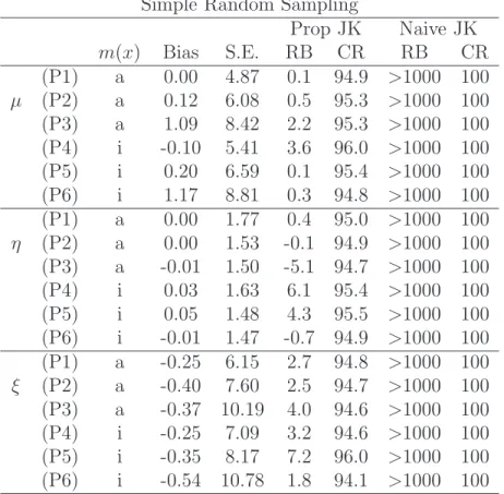
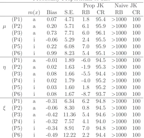
Tables 1 and 2 present the simulation results under simple random sam-pling and probability proportional to size samsam-pling, respectively, based on
2,000 Monte Carlo samples. Under both sampling designs, the nearest neigh-bor imputation estimator has small biases for all parameters µ, η and ξ, under (P1)–(P3) with m(x) accurate approximation for the mean function and (P4)–(P6) with m(x) inaccurate approximation of the mean function. For variance estimation, as expected, the naive jackknife variance estimator is severely biased, indicating that the lack of smoothness of the matching estimator needs to be taken into account in variance estimation. In contrast, the proposed jackknife variance estimators provide satisfactory results under both sampling designs and for all parameters. The relative biases are small and the empirical coverage rates are close to the nominal coverage. Overall, the simulation results suggest that the proposed variance estimator works reasonably well under the settings we considered.
6
Discussion
Instead of choosing the nearest neighbor as a donor for missing items, we can consider fractional imputation (Kim and Fuller; 2004; Yang and Kim; 2016) using K (K > 1) nearest neighbors. Such extension remains an interesting avenue for future research.
Appendix
The Appendix includes proofs of Theorems 1 and 2 and additional assump-tions.
Table 1: Simulation results for the population mean µ, the population pro-portionη= 0.8 and the population medianξunder simple random sampling: Bias (×102) and S.E. (×102) of the point estimator, Relative Bias of
jack-knife variance estimates (×102) and Coverage Rate (%) of 95% confidence intervals.
Simple Random Sampling
Prop JK Naive JK m(x) Bias S.E. RB CR RB CR (P1) a 0.00 4.87 0.1 94.9 >1000 100 µ (P2) a 0.12 6.08 0.5 95.3 >1000 100 (P3) a 1.09 8.42 2.2 95.3 >1000 100 (P4) i -0.10 5.41 3.6 96.0 >1000 100 (P5) i 0.20 6.59 0.1 95.4 >1000 100 (P6) i 1.17 8.81 0.3 94.8 >1000 100 (P1) a 0.00 1.77 0.4 95.0 >1000 100 η (P2) a 0.00 1.53 -0.1 94.9 >1000 100 (P3) a -0.01 1.50 -5.1 94.7 >1000 100 (P4) i 0.03 1.63 6.1 95.4 >1000 100 (P5) i 0.05 1.48 4.3 95.5 >1000 100 (P6) i -0.01 1.47 -0.7 94.9 >1000 100 (P1) a -0.25 6.15 2.7 94.8 >1000 100 ξ (P2) a -0.40 7.60 2.5 94.7 >1000 100 (P3) a -0.37 10.19 4.0 94.6 >1000 100 (P4) i -0.25 7.09 3.2 94.6 >1000 100 (P5) i -0.35 8.17 7.2 96.0 >1000 100 (P6) i -0.54 10.78 1.8 94.1 >1000 100
Prop JK: proposed jackknife variance estimation; Naive JK: naive jackknife variance estimation. a: accurate and i: inaccurate.
Table 2: Simulation results for the population mean µ, the population pro-portion η= 0.8 and the population median ξ under probability proportional to size sampling: Bias (×102) and S.E. (×102) of the point estimator,
Rel-ative Bias of jackknife variance estimates (×102) and Coverage Rate (%) of
95% confidence intervals.
Probability Proportional to Size
Prop JK Naive JK m(x) Bias S.E. RB CR RB CR (P1) a 0.07 4.71 1.8 95.4 >1000 100 µ (P2) a 0.20 5.71 6.1 95.9 >1000 100 (P3) a 0.73 7.71 6.0 96.1 >1000 100 (P4) i -0.06 5.29 2.4 95.5 >1000 100 (P5) i 0.22 6.08 7.0 95.9 >1000 100 (P6) i 0.99 8.23 5.4 95.1 >1000 100 (P1) a -0.01 1.89 -6.0 94.5 >1000 100 η (P2) a 0.02 1.63 -1.9 95.3 >1000 100 (P3) a 0.08 1.66 -5.5 94.4 >1000 100 (P4) i 0.02 1.79 -4.0 95.2 >1000 100 (P5) i 0.03 1.60 1.8 95.2 >1000 100 (P6) i 0.08 1.67 -8.7 93.7 >1000 100 (P1) a -0.31 6.34 6.2 94.8 >1000 100 ξ (P2) a -0.06 8.30 0.8 94.5 >1000 100 (P3) a -0.42 11.36 5.4 94.6 >1000 100 (P4) i -0.32 7.57 4.1 94.0 >1000 100 (P5) i -0.34 8.91 7.0 94.8 >1000 100 (P6) i -0.49 12.22 2.2 94.4 >1000 100
Prop JK: proposed jackknife variance estimation; Naive JK: naive jackknife variance estimation. a: accurate and i: inaccurate.
A7
Proof for Theorem 1
With a scalar matching variable m, we have
BN = n1/2 N X i∈A 1 πi (1−δi){µg(xi(1))−µg(xi)} ≤ n 1/2 N X i∈A 1 πi (1−δi)|mi(1)−mi |=op(1),
where ≤ in the second line follows by Assumption 3 (ii). Based on the decomposition in (5), we can write
n1/2(ˆµg,NNI−µg) =DN +op(1), (A1)
where DN is defined in (6). Then, to study the asymptotic properties of
n1/2(ˆµ
g,NNI−µg), we only need to study the asymptotic properties ofDN. For
simplicity, we introduce the following notation: µg,i =µg(xi)≡E{g(y)|xi}
and ei =g(yi)−µg,i. We express
DN = n1/2 N " X i∈A 1 πi {µg,i+δi(1 +ki)ei} − N X i=1 g(yi) # = n 1/2 N N X i=1 Ii πi −1 µg,i+ n1/2 N N X i=1 Ii πi δi(1 +ki)−1 ei, (A2)
and we can verify that the covariance of the two terms in (A2) is zero. Thus,
var(DN) = var ( n1/2 N N X i=1 Ii πi −1 µg,i ) +var " n1/2 N N X i=1 Ii πi δi(1 +ki)−1 ei # .
The first term, as n→ ∞, becomes
Vgµ = lim n→∞ n N2E ( varp X i∈A µg,i πi !) ,
and the second term, as n→ ∞, becomes Ve g = plim n N2 N X i=1 Ii πi δi(1 +ki)−1 2 var(ei |xi).
The remaining is to show that Ve
g =O(1). To do this, the key is to show that
the moments of ki are bounded. Under Assumption 2, it is easy to verify
that
ωk˜i ≤ki ≤ω¯˜ki, (A3)
for some constants ωand ¯ω, where ˜ki =Pjn=1(1−δj)dij is the number of unit
i used as a match for the nonrespondents. Under Assumption 3, ˜ki =Op(1)
and E(˜ki) and E(˜ki2) are uniformly bounded over n (Abadie and Imbens;
2006, Lemma 3); therefore, together with (A3), we have ki = Op(1) and
E(ki) and E(ki2) are uniformly bounded over n. Therefore, a simple algebra
yields Ve
g =O(1).
Combining all results, the asymptotic variance of n1/2(ˆµ
g,NNI − µg) is
Vµ
g +Vge. By the central limit theorem, the result in Theorem 1 follows.
A8
Proof for Theorem 2
We impose the following assumptions for the population parameter ξN and
the population estimating function SN(·); see also Wang et al. (2011).
Assumption A4 (i) The population parameter ξN lies in a closed interval
Iξ on R;
(iii) the population estimating function SN(ξ) converges to S(ξ) uniformly
on Iξ as N → ∞, and the equation S(ξ) = 0 has a unique root in the
interior of Iξ;
(iv) the limiting function S(ξ) is strictly increasing and absolutely continu-ous with finite first derivative inIξ, and the derivativeS′(ξ)is bounded
away from 0 for ξ in Iξ;
(v) the population quantities
sup ξ∈Is Nα|SN(ξN +N−αξ)−SN(ξN)−S(ξN +N−αξ)−S(ξN)| →0, and sup ξ∈Is N−1 N X i=1 |s(yi−ξN −N−αξ)−s(yi−ξN)|=Op(N−α),
where Is is a large enough compact set in R and α∈(1/4,1/2].
Assumption A4 (v) holds with probability one under suitable assumptions on the probability mechanism generating theyi’s and on the functions(·), and
therefore is justifiable. Under Assumption A4, by the standard arguments from the theory on M-estimators (Serfling; 1980), ˆξNNI is consistent for ξN.
We further make the following assumption.
Assumption A5 The nearest neighbor imputation estimator ξˆNNI is root-n
consistent for ξN,
Now, we give proof for Theorem 2. Under Assumptions A4 and A5, we can write
ˆ
SNNI( ˆξNNI)−SN(ξN) ={SˆNNI(ξN)−SN(ξN)}+S
′
(ξN)( ˆξNNI−ξN) +op(n
−1/2
).
By Assumption A4 (iv), S(ξ) is smooth, and therefore SN(ξN) = Op(N−1),
ˆ
SNNI( ˆξNNI) = Op(n−1), and the left hand side of (A4) isop(n−1/2). Therefore,
we can obtain a linearization for ˆξNNI as in (9).
Based on the linearization (9), the asymptotic varianceVξ = ˙S(ξ)−2var{SˆNNI(ξ)}.
Following a similar derivation in the proof for Theorem 1, it is easy to show that var{SˆN(ξ)}= lim n→∞ n N2E varp " X i∈A E{s(yi−ξ)|xi} πi #! + plim n N2 N X i=1 Ii πi δi(1 +ki)−1 2 var [s(yi−ξ)−E{s(yi−ξ)|xi} |xi].
A9
Assumptions
Assumption A6 The following conditions hold for kernel functionK(·)and bandwidth h:
(i) the kernel functionK(·)is absolutely continuous with nonzero finite deriva-tive K′
(·) and ´
K(x)dx= 1;
(ii) the bandwidth h→0 and nh→ ∞ as n → ∞;
(iii) there exists a constant c, such that |h−1K′
(x1/h) − h−1K′(x2/h)| ≤ c|x1−x2| for any x1, x2 and h arbitrarily small.
Assumption A6 states conditions on the smoothness and tail behavior of the kernel functions. Popular kernel functions, including Epanechnikov, Gaussian, and triangle kernels, satisfy the required conditions.
References
Abadie, A. and Imbens, G. W. (2006). Large sample properties of matching estimators for average treatment effects, Econometrica 74: 235–267. Berger, Y. G. and Skinner, C. J. (2003). Variance estimation for a low
in-come proportion,Journal of the Royal Statistical Society: series C (applied statistics) 52: 457–468.
Chen, J. and Shao, J. (2000). Nearest neighbor imputation for survey data,
J. Offic. Stat. 16: 113–131.
Chen, J. and Shao, J. (2001). Jackknife variance estimation for nearest-neighbor imputation, J. Amer. Statist. Assoc. 96: 260–269.
Deville, J. C. (1999). Variance estimation for complex statistics and estima-tors: linearization and residual techniques, Surv. Methodol.25: 193–204. Francisco, C. A. and Fuller, W. A. (1991). Quantile estimation with a
com-plex survey design, Ann. Statist. 19: 454–469.
Fuller, W. A. (2009). Sampling Statistics, Wiley, Hoboken.
Isaki, C. T. and Fuller, W. A. (1982). Survey design under the regression superpopulation model, J. Amer. Statist. Assoc. 77: 89–96.
Kim, J. K. and Fuller, W. A. (2004). Fractional hot deck imputation,
Biometrika91: 559–578.
nearest neighbor imputation for US Census long form data,The Annals of Applied Statistics5: 824–842.
Kim, J. K., Navarro, A. and Fuller, W. A. (2006). Replication variance estimation for two-phase stratified sampling, J. Amer. Statist. Assoc.
101: 312–320.
Lee, H. and S¨arndal, C. E. (1994). Experiments with variance estimation from survey data with imputed values, J. Offic. Stat. 10: 231–243.
Otsu, T. and Rai, Y. (2016). Bootstrap inference of matching estimators for average treatment effects, J. Amer. Statist. Assoc.
p. DOI:10.1080/01621459.2016.1231613.
Rust, K. F. and Rao, J. N. K. (1996). Variance estimation for complex surveys using replication techniques, Stat Methods Med Res 5: 283–310. Sande, I. G. (1979). A personal view of hot deck imputation procedures,
Surv. Methodol.5: 238–258.
Serfling, R. J. (1980). Approximation Theorems of Mathematical Statistics, Hoboken, NJ: Wiley.
Shao, J. and Steel, P. (1999). Variance estimation for survey data with com-posite imputation and nonnegligible sampling fractions, J. Amer. Statist. Assoc. 94: 254–265.
Shao, J. and Wang, H. (2008). Confidence intervals based on survey data with nearest neighbor imputation, Statist. Sinica 18: 281–297.
Wang, J. C., Opsomer, J. D. et al. (2011). On asymptotic normality and vari-ance estimation for nondifferentiable survey estimators,Biometrika98: 91– 106.
Wolter, K. (2007). Introduction to Variance Estimation, 2 edn, Springer, New York.
Wu, C. and Sitter, R. R. (2001). A model-calibration approach to using complete auxiliary information from survey data, J. Amer. Statist. Assoc.
96: 185–193.
Yang, S. and Kim, J. K. (2016). Fractional imputation in survey sampling: A comparative review, Statist. Sci. 31: 415–432.