River Discharge and Water Quality
M. J. Kingdon, H. A. Bootsma, J. Mwita, B. Mwichande
SADC/GEF Lake Malawi/Nyasa Biodiversity Conservation Project,
P.O.Box 311, Salima, Malawi.
R.E. Hecky
Environment Canada, National Water Research Institute, P.O. Box 5050
Burlington, ON L7R 4A6 Canada
Introduction
The Lake Malawi/Nyasa Biodiversity Conservation Project has the objectives of determining the conditions essential for the maintenance of the lake’s unique biodiversity and recommending strategies for conserving those conditions. One essential condition for sustaining aquatic life and biodiversity is maintenance of good water quality. Rivers provide an important connection between the waters of Lake Malawi and its surrounding land area. Land use, topography and population density may affect the transport of nutrients and sediments in the rivers and may influence lake-wide biological activity and water quality. Within the project, river studies have been implemented to:
• Understand how river basin characteristics such as topography, population density and regional climate influence water quality and river-flow characteristics.
• Determine the annual loading of nutrients and sediments from rivers for inclusion in the whole-lake nutrient budget.
• Assess the current water quality of in-flowing rivers, especially for parameters such as phosphorus, nitrogen, silica and suspended solids that are most likely to affect the limnology of the lake and its biodiversity.
• Suggest sensitive chemical parameters that are particularly important to the lake’s water quality and biodiversity and which should be the focus of future monitoring/research programs.
Establishing a lake-wide budget of available nutrients is essential for understanding the role that these nutrients play in primary productivity and ecosystem function. To date, there has been limited attention given to the importance of these constituents carried to Lake Malawi in river water and their effect on the lake-wide budget. Previous estimates of river nutrient and sediment loading have been established using single samples from a limited number of Malawian rivers (Bootsma & Hecky, 1993). Although these estimates do give an indication of river chemistry, they do not provide information on the temporal dynamics that may influence the annual loading of nutrients to the lake. Distinct rainy and dry seasons in the lake watershed result in large seasonal changes in river discharge. Increasing our understanding of how river chemistry responds to short term and seasonal changes in river discharge is fundamental in determining the annual loading of nutrients to the lake from rivers.
Spatial variations of rainfall, topography and land-use may also affect the availability of nutrients in river water; therefore it is useful to compare nutrient loading on a regional basis, and to assess possible impacts of human development in the catchment area. The influence of agricultural development, deforestation, biomass burning, and human settlement have been shown to affect water runoff and chemistry (Calder et al, 1995) and are important to address in nutrient loading studies. The purpose of the river sampling program is to establish a more detailed understanding of river chemistry, its temporal and regional variations, and how it may relate to land use and basin characteristics. This
chapter presents data on river water chemistry, temperature, suspended solids, and discharge. Data on contaminants in river water are presernted in Chapter 9 (Kidd et al.).
Methods
River Sampling.
Given the size of Lake Malawi/Nyasa and the remoteness of many of its inflows,
the selection of rivers to be sampled was based largely on their accessibility and proximity to the Senga Bay research laboratory. Most of the major inflows on the western (Malawian) shore of the lake were sampled throughout the period from late 1996 to early 1998, covering the full extent of one annual flow season. This typically begins in early December at the onset of the rainy season.Frequent samples from Tanzanian rivers were not available until the 1998/99 rainy season. Data for these samples were not available at the time of writing this report. They will be presented in later publications. No samples were taken in Mozambique, which represents a small portion of the lake watershed. Although there were a number of major inflows that were not sampled during 1996-98, including several large rivers on the north and northeastern shore in Tanzania, the sampled rivers encompass a large portion of the total watershed and include regions of varying rainfall, topography and human development. This provides a range of catchment characteristics that are typically found throughout the entire lake basin.
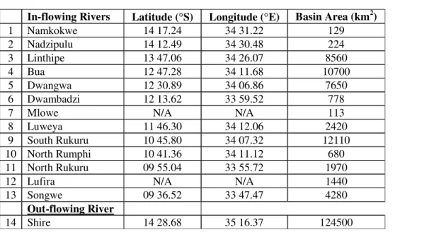
Most rivers were sampled at their intersection with the lakeshore highway, typically no more than a few kilometers from the lake inlet (figure 2.0 & table 2.0). Although some small chemical changes may occur downstream of the sampling points, the locations do allow for samples that describe water chemistry from the vast majority of each river basin, and are assumed to be indicative of water that is flowing directly into the lake.
River sampling was integrated into the lake-wide water quality monitoring program, and was performed as frequently as time permitted. Samples were taken from rivers closest to Senga Bay on a weekly basis, and on a monthly schedule for the more distant northern rivers. More frequent samples were obtained after December 1997, and included 3 samples per week from the Linthipe River, and one sample per week each from the Bua, Dwangwa, Namkokwe, and Nadzipulu Rivers. All other rivers were sampled approximately once per month.
Samples were obtained either by filling bottles from the river’s edge, by wading, or by lowering a plastic bucket from the bridge, depending on the conditions at each site. At all locations, care was taken to obtain samples from well-mixed water that was indicative of the total flow of the river. In most rivers, water depth was less than one meter deep across the entire channel and flow was very turbulent, thereby facilitating the easy collection of a representative sample. However, no attempt was made to sample the bed load (courser grain material in partial suspension near the bottom of the river) because the bed load is unlikely to be widely distributed in the lake beyond the receiving river delta (Johnson, 1990). Both the bottles and bucket were rinsed twice with river water before obtaining the final sample. Samples were kept cool (<10°C) and transported to Senga Bay for filtration and analysis. Filtration was usually completed immediately after sampling, in accordance with procedures outlined in “The Chemical Analysis of Fresh Water” (Stainton et al. 1977).
Sample Analysis. Sample analysis was carried out both at the Senga Bay laboratory and in Winnipeg, Manitoba at the Freshwater Institute (Department of Fisheries and Oceans). All analyses were performed as outlined in Stainton et al (1977). Analyses carried out in Senga Bay include total suspended solids (TSS), nitrate (NO3-), ammonium (NH4+), soluble reactive phosphorus (SRP),
soluble reactive silica (SRSi), total dissolved nitrogen (TDN) and total dissolved phosphorus (TDP). Analyses carried out in Winnipeg include dissolved organic carbon (DOC), suspended nitrogen (SUSPN),
Figure 2.0 Geographic location of rivers with available chemistry and river flow data, and the Ruhuhu river, the lake’s largest inflow (chemistry and flow data not yet available).
Table 2.0. Rivers with available chemistry and flow data used in this report.
In-flowing Rivers Latitude (°S) Longitude (°E) Basin Area (km2)
1 Namkokwe 14 17.24 34 31.22 129 2 Nadzipulu 14 12.49 34 30.48 224 3 Linthipe 13 47.06 34 26.07 8560 4 Bua 12 47.28 34 11.68 10700 5 Dwangwa 12 30.89 34 06.86 7650 6 Dwambadzi 12 13.62 33 59.52 778
7 Mlowe N/A N/A 113
8 Luweya 11 46.30 34 12.06 2420
9 South Rukuru 10 45.80 34 07.32 12110
10 North Rumphi 10 41.36 34 11.12 680
11 North Rukuru 09 55.04 33 55.72 1970
12 Lufira N/A N/A 1440
13 Songwe 09 36.52 33 47.47 4280
Out-flowing River
14 Shire 14 28.68 35 16.37 124500
phosphorus (SUSPP), carbon (SUSPC), iron (SUSPFe), silica (SUSPSi) and dissolved sulphate (SO4
2-). Analysis of some TDN and TDP samples was also performed in Winnipeg. All dissolved nutrient samples were immediately frozen after filtration and thawed prior to analysis in Senga Bay. Dissolved nutrient samples transported to Winnipeg were preserved with mercuric chloride prior to shipping. NO3- and NH4+ results were summed to obtain the dissolved inorganic nitrogen (DIN) estimates
outlined in this report. Samples collected in the 1996/97 rainy season were also analyzed for major ions, but these results are not reported here.
Determining Total Lake Inflow.
This report makes extensive use of the World Meteorological Organization’s Water Resources Evaluation of Lake Malawi (Kidd 1983). It is the only known report that provides long term river discharge data (from Malawi, Mozambique and Tanzania) and summarizes river inflows by region and river basin. Therefore, it is a very useful guide when making assumptions about river inflow from areas of the catchment for which there are presently no data.
Daily river discharge records were obtained for the major rivers used in this report from the Malawi Water Department. Flows are reported as the average of two daily measurements taken from a staff gauge for rivers with a known stage/discharge relationship. The Water Department reports periodic calibration of the stage/discharge relationships. All flow data are taken from monitoring stations close to the lake, within a few kilometers of the lakeshore.
The period of collected river discharge data extends from November 1996 to early 1998 for most rivers. This makes it possible to study the seasonal trends in river discharge over the course of an entire flow season and to calculate the total annual inflow from the sampled rivers. Data from the period of January 1, 1997 to December 31, 1997 were selected for the calculation of annual discharge and nutrient flux. Although this time span does not correspond precisely to the hydrologic year (which usually commences in early December), it was chosen because it allows for the inclusion of data collected during December 1997, when sampling was more spatially and temporally complete than during 1996.
Discharge records for the Namkokwe and South Rukuru Rivers were not available beyond December 1, 1997. Therefore, the annual input from these rivers is reported from November 1,1996 to November 30, 1997. This is not expected to have a significant impact on estimates of lake inflow and nutrient loading because this period encompasses one full flow season, chemistry data are
available for the entire period, and the inflow from these rivers is relatively small when compared to the entire lake watershed.
Kidd (1983) divides the catchment area into 20 sections, of which 11 are single river basins, and 9 are regions containing more than one river (figure 2.1 & table 2.1). Of the 11 river basins, discharge records in this report have been collected for 9 of them, including the Linthipe, Bua, Dwangwa, Luweya, South Rukuru, North Rumphi, North Rukuru, Lufira and Songwe Rivers. The remaining two, the Kiwira and Ruhuhu Rivers, are in Tanzania, from where discharge records could not be obtained in time for inclusion in this report.
The Mlowe, Dwambadzi, Namkokwe, and Nadzipulu Rivers, for which discharge records are available, are not reported as individual basins in the Kidd report, but are included in larger regions containing more than one river as follows:
• Namkokwe and Nadzipulu (part of the Mtakataka lakeshore region),
• Dwambadzi and Mlowe (part of the Dwambadzi lakeshore region).
In this manner, river discharge data (for entire or partial regions) is available from 11 of the 20 river basins/regions surrounding Lake Malawi as outlined in Kidd (1983).
In order to estimate the volume of water entering the lake from areas with no or partial discharge data, 2 methods were used:
1) For regions with partial data (Mtakataka and Dwambadzi lakeshore regions):
The runoff (in mm) for the known rivers in the region was calculated from 1997 daily discharge data. This runoff was then applied to the entire region. For example, in the Dwambadzi lakeshore region, the annual volume (V) of water discharged from the Dwambadzi and Mlowe Rivers was totaled, then runoff (Depth: D) was calculated over the known catchment area (A) of the 2 rivers, following equation 1.
D(373mm)=V(332343000m3)/A(891000000m2)x1000 (1)
The calculated annual runoff (D) was then applied to the area of the entire Dwambadzi lakeshore region (A) to estimate the total volume of water entering the lake (V) following equation 2.
V(.7087km3)=D(373mm)/1000000xA(1900km2) (2)
2) For regions with no discharge records (such as the Ruhuhu River and Eastern Lakeshore).
The total inflow volume was estimated by comparing the long-term average runoff in the region as reported by Kidd (1983) with the runoff from adjacent regions for which flow records were available in 1997. These comparisons were made under the assumption that regional rainfall, and therefore runoff, would be similar among adjacent basins with similar basin morphology.
The long-term average runoff reported by Kidd for each region provides a useful guide to determining the inflow from regions with no river discharge data. The calculated runoff (from 1997) in several adjacent regions was compared to long-term average runoff in those same regions in order to determine if a larger or smaller amount of runoff was observed. The percent difference of the calculated 1997 runoff and long-term average was then applied to the region with no river discharge data. The percent difference was weighted according to the area of the adjacent basins such that the larger of the adjacent basins used in determining the percent difference exerted a greater influence on the final calculation. The average runoff difference (in adjacent basins) was weighted under the assumption that the larger areas will experience rainfall (and therefore runoff) that is more characteristic of the entire region used in the comparison. An example of the calculation procedure follows:
• When determining the total inflow from the Usisya lakeshore region, the calculated 1997 runoff in the adjacent Luweya, South Rukuru and North Rumphi River basins was used in the table below (c). The calculated runoff values were compared to long-term averages in each region (b). The weighted percent difference (e) was applied to the long-term average runoff in the Usisya region (Kidd, 1983) to estimate annual runoff in 1997. This estimated runoff was then applied to the area of the Usisya region in order to determine total water inflow volume.
River/ Region Basin area (km2) (a) Long-term average runoff (mm) (b) Calculated 1997 runoff (mm) (c) Difference (d) = (c/b) Weighted Difference (e)=(a/13911x d) Luweya 1428 480 173 .36 0.037 S Rukuru 11800 100 38 .38 0.325 N Rumphi 683 670 462 .69 0.033 13911 (total) 0.4 (total)
• Usisya Lakeshore long-term average runoff = 270mm Estimated 1997 runoff = 270mm x 0.4 = 108mm Total inflow = 108mm/1000000 x 1430 km2 = 0.15 km3
An annual catchment inflow was established using the above methods to estimate the inflow from regions with no or partial river discharge data. A summary of the calculations used for each region is outlined in table 2.2.
Figure 2.1. Geographic locations of the individual catchment regions in portions A, B, and C (from Kidd, 1983).
Lake
Table 2.1. Inflow regions used in the annual inflow and nutrient/sediment loading calculations, and portions A, B, and C in regional summaries (Kidd, 1983).
Region Name Area (km2) 1997 data available?
Southern Lakeshore 3,100 Mtakataka Lakeshore 1,760 9 Linthipe 8,560 9 Nkotakota Lakeshore 4,940 Bua 10,700 9 Dwangwa 7,650 9 Dwambadzi Lakeshore 1,900 9 Luweya 2,420 9 Usisya Lakeshore 1,430 South Rukuru 12,110 9 North Rukuru 680 9 Karonga Lakeshore 2,270 North Rukuru 1,970 9 Lufira 1,440 9 Songwe 4,280 9 Kiwira 1,690 Northern Lakeshore 2,290 Northeastern Lakeshore 4,330 Ruhuhu 14,070 Eastern Lakeshore 8,160 Total 95,740 Total in Malawi 65,200
Total Area Sampled 53,470
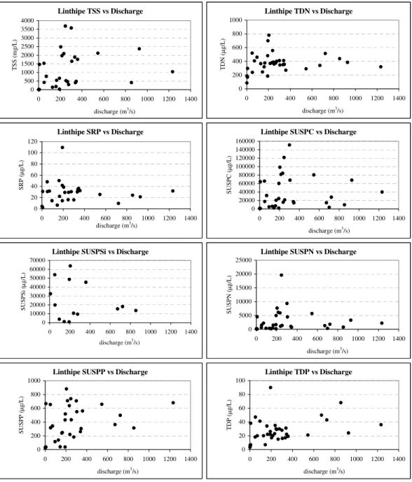
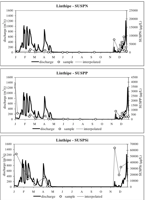
Investigating the Relationship between River Discharge and Nutrient Concentration. For all rivers and nutrients, the relationship between daily river discharge and nutrient concentration was examined to determine if nutrient concentrations could be estimated as a function of discharge. For all rivers and nutrients, no statistically valid relationship was found that could be applied to the data (figure 2.2). However, when both discharge and nutrient concentration were plotted against time, several trends emerged. For all in-flowing rivers, the early part of the flow season (December) exhibited a flushing effect for most nutrients, whereby high concentrations were found in river water just as flow increased at the beginning of the rainy season. These trends were especially evident for particulate nutrients (figure 2.3). Concentrations for most nutrients generally diminished as the flow season progressed, but maintained a positive correlation with flow (especially for particulates). There was no indication of strong dilution in any of the rivers (decreased concentration with increased flow). The high concentrations at the beginning of the flow season prevented the establishment of a consistent relationship between flow and discharge. A lack of data prevented the use of shorter time spans (such as months) when testing the discharge/concentration comparison that may have reduced the influence of seasonal signals apparent in the data. For these reasons, a discharge/nutrient concentration relationship could not be effectively applied to the data to determine nutrient loading.
Although the frequency of sampling was inadequate to assess daily changes in nutrient concentration, seasonal fluctuations were apparent for most nutrients in all rivers (figure 2.4). Therefore, daily nutrient concentrations were estimated by interpolating between sample dates. If no
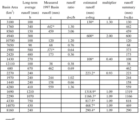
Table 2.2. Regional runoff calculations summary (see text for method of estimating).
Long-term Measured runoff estimated multiplier runoff Basin Area average 1997 Basin ratio runoff summary
(km2) runoff (mm) runoff (mm) (mm) (mm) a b c d=c/b e=bxg g f=c&e Southern lakeshore 3100 100 130* 1.30 130 Mtakataka lakeshore 1760 340 442* 1.30 442 Linthipe 8560 150 459 3.06 459 Nkotakota lakeshore 4940 300 600* 2.00 600 Bua 10700 100 120 1.20 120 Dwangwa 7650 90 68 0.76 68 Dwambadzi lakeshore 1900 580 373* 0.64 373 Luweya 2420 480 173 0.36 173 Usisya lakeshore 1430 270 108* 0.40 108 South Rukuru 12110 100 38 0.38 38 North Rumphi 680 670 462 0.69 462 Karonga lakeshore 2270 240 223.2* 0.93 223 North Rukuru 1970 240 244 1.02 244 Lufira 1440 240 158 0.66 158 Songwe 4280 410 559 1.36 559 Kiwira 1690 1210 1318.9* 1.09 1319 Northern lakeshore 2290 1070 1166.3* 1.09 1166 Northeast lakeshore 4330 750 817.5* 1.09 818 Ruhuhu 14070 430 468.7* 1.09 469 Eastern lakeshore 8160 240 290.4* 1.09 290 continued… runoff calculation notes*
Southern lakeshore based on runoff ratio (d) from #2.
Mtakataka lakeshore based on total measured runoff from Namkokwe and Nadzipulu rivers (442 mm over 353 km2) Linthipe measured runoff
Nkotakota lakeshore based on the area weighted average runoff ratio from regions 3 & 5.
Bua measured runoff
Dwangwa measured runoff
Dwambadzi lakeshore based on total measured runoff from Dwambadzi and Mlowe rivers (373mm from 891 km2) Luweya measured runoff
Usisya lakeshore based on the area weighted average runoff ratio from regions 8,10 & 11. South Rukuru measured runoff
North Rumphi measured runoff
Karonga lakeshore based on the area weighted average runoff ratio from regions 11 & 13. North Rukuru measured runoff
Lufira measured runoff Songwe measured runoff
Kiwira based on the area weighted average runoff ratio from regions 11,13,14 & 15. Northern lakeshore based on the area weighted average runoff ratio from regions 11,13,14 & 15. Northeast lakeshore based on the area weighted average runoff ratio from regions 11,13,14 & 15. Ruhuhu based on the area weighted average runoff ratio from regions 11,13,14 & 15. Eastern lakeshore based on the area weighted average runoff ratio from regions 11,13,14 & 15.
Figure 2.2 Example plots of nutrient concentration vs. discharge on the day of sampling for various parameters. No statistically valid relationships could be found.
Linthipe TSS vs Discharge 0 500 1000 1500 2000 2500 3000 3500 4000 0 200 400 600 800 1000 1200 1400 discharge (m3/s) T SS ( m g/ L ) Linthipe TDN vs Discharge 0 200 400 600 800 1000 0 200 400 600 800 1000 1200 1400 discharge (m3/s) TD N ( µ g/ L ) Linthipe SRP vs Discharge 0 20 40 60 80 100 120 0 200 400 600 800 1000 1200 1400 discharge (m3/s) SR P ( µ g/ L )
Linthipe SUSPC vs Discharge
0 20000 40000 60000 80000 100000 120000 140000 160000 0 200 400 600 800 1000 1200 1400 discharge (m3/s) SU SPC ( µ g/ L )
Linthipe SUSPSi vs Discharge
0 10000 20000 30000 40000 50000 60000 70000 0 200 400 600 800 1000 1200 1400 discharge (m3/s) SUSPSi ( µ g/L )
Linthipe SUSPN vs Discharge
0 5000 10000 15000 20000 25000 0 200 400 600 800 1000 1200 1400 discharge (m3/s) SU SPN ( µ g/ L )
Linthipe SUSPP vs Discharge
0 200 400 600 800 1000 0 200 400 600 800 1000 1200 1400 discharge (m3/s) SU SPP ( µ g/ L ) Linthipe TDP vs Discharge 0 20 40 60 80 100 0 200 400 600 800 1000 1200 1400 discharge (m3/s) TD P ( µ g/ L )
Figure 2.3 Examples of seasonal nutrient sample concentrations at various points in the annual hydrographs and seasonal cycle. High suspended nutrient concentrations are found in the early flow season (November through January).
Linthipe - SUSPN 0 200 400 600 800 1000 1200 1400 1600 J F M A M J J A S O N D di sc ha rge (m 3 /s) 0 5000 10000 15000 20000 25000 SUSPN ( µ g/ L)
discharge sample interpolated Linthipe - SUSPP 0 200 400 600 800 1000 1200 1400 1600 J F M A M J J A S O N D dis char ge ( m 3 /s ) 0 500 1000 1500 2000 2500 3000 3500 4000 4500 SUSPP ( µ g/L )
discharge sample interpolated Linthipe - SUSPSi 0 200 400 600 800 1000 1200 1400 1600 J F M A M J J A S O N D dis char ge ( m 3 /s ) 0 10000 20000 30000 40000 50000 60000 70000 SUSPSi ( µ g/L )
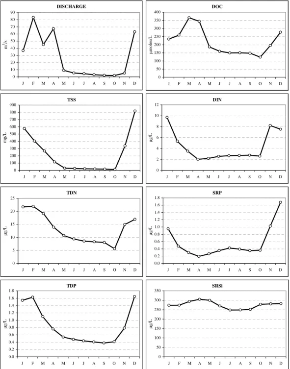
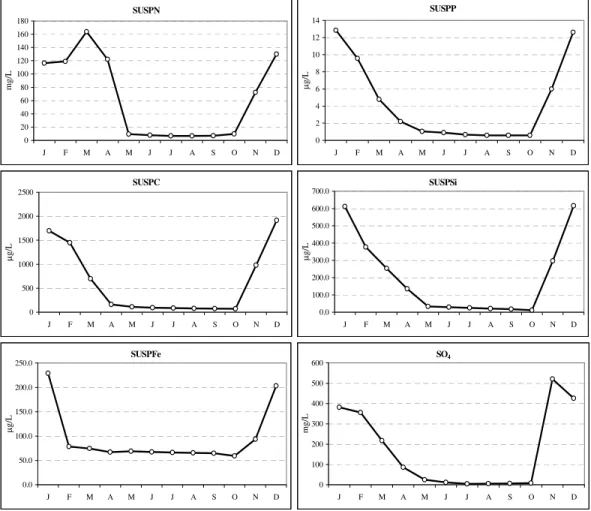
Figure 2.4 Mean monthly nutrient and sediment concentrations in rivers with available sample data. DISCHARGE 0 10 20 30 40 50 60 70 80 90 J F M A M J J A S O N D m 3/s DOC 0 50 100 150 200 250 300 350 400 J F M A M J J A S O N D µ moles/L TSS 0 100 200 300 400 500 600 700 800 900 J F M A M J J A S O N D mg/L DIN 0 2 4 6 8 10 12 J F M A M J J A S O N D µ g/L TDN 0 5 10 15 20 25 J F M A M J J A S O N D µ g/L SRP 0.0 0.2 0.4 0.6 0.8 1.0 1.2 1.4 1.6 1.8 J F M A M J J A S O N D µ g/L TDP 0.0 0.2 0.4 0.6 0.8 1.0 1.2 1.4 1.6 1.8 J F M A M J J A S O N D µ g/L SRSi 0 50 100 150 200 250 300 350 J F M A M J J A S O N D µ g/L
Figure 2.4 continued.
nutrient data were available for a river at the end of the fry season, the last measured nutrient concentrations for the dry season were applied up until the date that discharge began to increase in the
SUSPN 0 20 40 60 80 100 120 140 160 180 J F M A M J J A S O N D mg/L SUSPP 0 2 4 6 8 10 12 14 J F M A M J J A S O N D µ g/L SUSPC 0 500 1000 1500 2000 2500 J F M A M J J A S O N D µ g/L SUSPSi 0.0 100.0 200.0 300.0 400.0 500.0 600.0 700.0 J F M A M J J A S O N D µ g/L SUSPFe 0.0 50.0 100.0 150.0 200.0 250.0 J F M A M J J A S O N D µ g/L SO4 0 100 200 300 400 500 600 J F M A M J J A S O N D mg/L
following rainy season, after which nutrient concentrations were interpolated to the values measured on the first sample date in the rainy season. Multiplying nutrient concentration by flow produced loading estimates on a daily basis. Daily rates were then summed to derive an annual total. The results are considered to be more accurate than previous estimates (Bootsma & Hecky 1993; Bootsma
et al. 1995) which applied average annual nutrient concentrations.
For rivers with no nutrient data available for the first few months of 1997, mean nutrient concentrations from January 1998 (a period of more frequent sampling) were used to approximate nutrient concentration in early 1997. It is assumed that this will approximate the actual loading during the early portion of the flow season more accurately than extending the dry season values from mid 1997 back to the beginning of the 1997 flow season. These manipulations were used for only a few rivers where the nutrient data set was limited. In most rivers, and for most nutrients, the standard linear interpolation was sufficient to estimate the temporal variations in nutrient concentration.
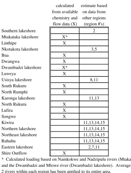
Determining Annual Loading from all In-flowing Rivers/Regions. Similar to the annual water discharge calculations, annual nutrient loading was calculated according to the regions outlined in Kidd (1983). For regions that did not have chemistry data, assumptions were made to approximate the loading from each area.
Nutrient loading from regions/rivers with no nutrient data was estimated from other basins with available data. Basins/regions were compared based on their proximity to each other and general physiographic features (population density and topography). These comparisons were very general in the absence of detailed land-use and physiographic data. Nevertheless, attempts were made to compare basins with others having similar features that may influence nutrient loading. For regions having available chemistry data, volume-weighted mean nutrient concentrations were calculated.
When applying normalized chemistry data from one region to another, attempts were made to include the data from several regions that have similar characteristics. The volume-weighted mean nutrient concentration from all similar regions was calculated and applied to the region without chemistry data. This reduces the error associated with including rivers with limited sample data, while accounting for various physiographic features that may be present in several different basins. For example, when estimating the nutrient load from the Ruhuhu River basin, the nutrient concentrations from the North Rumphi, North Rukuru, Lufira and Songwe Rivers were used. The Ruhuhu basin is characterized by moderate population density, with steep slopes and native vegetation mixed with agriculture and deforestation on the lower slopes. The rivers chosen for comparison are under the influence of similar regional climate, and all have steep slopes in the upper parts of their basins. Land-use ranges from the mostly undisturbed, pristine North Rumphi River, to the moderately cultivated Lufira and North Rukuru to the more densely populated and developed Songwe River basins. In order to provide an estimate of the potential error associated with applying nutrient concentrations from adjacent basins, the maximum and minimum annual volume-weighted nutrient concentrations (for each nutrient from the 4 rivers) was also applied to the Ruhuhu to give a maximum and minimum estimate of loading.
For the 2 regions that had only partial chemistry data (data existed for only 2 rivers within each region), the annual nutrient load from the rivers within each region was determined and multiplied by the ratio of (discharge for the entire region) : (discharge for the measured rivers). This was used when determining the nutrient load from the Mtakataka Lakeshore and Dwambadzi lakeshore regions.
A summary of nutrient load calculation procedures for each region is given in Table 2.3. 1997 catchment loading estimates were made by summing the annual nutrient loads from each region. Flow Variability Analysis. In addition to the analysis of water chemistry and loading, the variability of river discharge was examined for each river with available records in an attempt to assess the impact of catchment characteristics on river flow. Four measures of flow variability were utilized: three spread measures (.5S, .6S and .8S); and the coefficient of variation of the log of flows (CVLF5). This procedure follows that used for the Laurentian Great Lakes tributaries by Richards, (1990).
Table 2.3. Regional nutrient loading calculations summary. Loading from regions without sample data
was estimated from other regions with similar catchment characteristics (see text for details).
All measures of variability incorporate the use of percentile flows which give the daily discharge below which a given percent of measured values were measured. For example, if the value for the 25th
percentile is 100 m3 s-1, then 25% of measured discharge rates are ≥100. The spread measures are in the form of (qx-qy)/qm where qx corresponds to flow at percentile x, qy is the flow at percentile 100-x,
and qm is the median flow. The “fourth” spread (.5S) refers to the difference between the 75th and 25th
percentile, the .6S uses the 80th and 20th, and the .8S utilizes the 90th and 10th percentile. All spread measures are independent of scale and analogous to the coefficient of variation of daily average flows. The CVFL5 measure corresponds to the coefficient of variation of the logs of the average daily flows at the percentiles: {5, 10, 15,……,85,90,95}. It is scale dependent, thereby affected by the average daily discharge in each basin and the units of flow measure, which are m3 s-1 for all measures
in this report. Basins with lower average daily discharge will have higher CVFL5 values than basins
calculated estimate based
from available on data from chemistry and other regions
flow data (X) (region #'s)
Southern lakeshore 2 Mtakataka lakeshore X* Linthipe X Nkotakota lakeshore 3,5 Bua X Dwangwa X Dwambadzi lakeshore X* Luweya X Usisya lakeshore 8,11 South Rukuru X North Rumphi X Karonga lakeshore 11,13 North Rukuru X Lufira X Songwe X Kiwira 11,13,14,15 Northern lakeshore 11,13,14,15 Northeast lakeshore 11,13,14,15 Ruhuhu 11,13,14,15 Eastern lakeshore 2,7,11 Shire Outflow X
* Calculated loading based on Namkokwe and Nadzipulu rivers (Mtakataka lakeshore) and the Dwambadzi and Mlowe river (Dwambadzi lakeshore). Average loading from the 2 rivers within each region has been applied to its entire area.
with higher average discharge and similar flow distribution because of this scale dependence. However, the CVFL5 is a multi-point measure, and represents the range of data more accurately than the spread measures.
Both the spread and CVFL5 indices are considered well suited for rivers with near zero flows during a part of the annual cycle such as those in this report. Because daily discharge records are calculated from stage/discharge curves, and are not directly measured, many records positive discharge values on days when there was actually no flow. For this reason, and because CVFL5 is undefined at zero, all records of flow less than 0.1 m3/s have been excluded from the calculations.
Indices of flow variability were calculated for all rivers with available daily flow data. This includes one full flow season (1997) for the Namkokwe, Nadzipulu, Dwambadzi, Mlowe, Luweya, South Rukuru, North Rumphi, North Rukuru, Lufira and Songwe Rivers, and the period covering 1990 to 1998 for the Linthipe, Bua and Dwangwa Rivers. The measures of flow variability are best suited to long term data, thereby reducing the error associated with annual fluctuations, but are used in this report to highlight potential differences between river basins. The longer-term data for the Linthipe, Bua and Dwangwa Rivers will provide reference to the annual variability of the measures. Density-Dependent River Inflow Distribution. The impact of river-borne nutrients on the lake and its biota varies depending on the depth to which these nutrients sink after entering the lake. Nutrients that are retained and recycled within surface waters will be available for use by algae and bacteria, whereas nutrients that sink below the epilimnion may either slowly mix back into surface waters, or become permanently lost to burial in the deep sediments. To determine the relative importance of these pathways, a simple model was used to predict the depth to which river water will sink to after entering the lake. River water density was calculated using water temperature, conductivity and total suspended solids measurements from samples taken throughout the study period. The resulting density figures for each sample were then compared with lake water density.
Lake water density was calculated using temperature and conductivity vertical profile data collected with an automated Conductivity, Temperature and Depth (CTD) profiler (SeaBird SBE19). TSS was not included in the calculations because it is very low in lake water (Hecky & Bugenyi, 1992). Profiles were made on a monthly basis at the standard station (Station 900) northeast of the Senga Bay lab site. To calculate density, measured conductivity was first corrected for temperature and pressure, using the relationships described by Wüest et al. (1996) that aply to the average major ion composition of Lake Malawi/Nyasa water. Salinity was then determined as a function of conductivity, using the formula of Wüest et al. (1996). Density was determined from salinity using the formula of Chen and Millero (1986).
River density values were compared with CTD data for the same month of sampling at each depth in the profile. The depth strata at which river and lake water densities matched (closest) determined the depth at which river water is assumed to move to after entering the lake. Depth was calculated for each sample and average values for each river were determined to compare data between basins.
This model assumes that CTD data collected at Station 900 is indicative of lake water near the mouth of each river. Although there is undoubtedly spatial variation in the thermal structure of the lake, this variation is smaller than the seasonal variation in thermal structure recorded at Station 900, and therefore the use of CTD data from Station 900 still permits an assessment of the general trends in the vertical distribution of river water entering the lake. A more detailed analysis of plume dynamics for the Linthipe River has been carried out by G. McCullough and is presented as an annex to this chapter.
Results and Discussion
1997 Catchment Inflow. The whole-lake river inflow is summarized in table 2.4 which compares the 1997 calculated inflow with the long term averages reported by Kidd (1983). The 1997 inflow is
Table 2.4. Summary of lake inflows and outflows. The 1997 estimate is compared to the long-term average calculated by Kidd (1983).
Figure 2.5. Lake level variability during the study period. Significant increases in lake level followed large early season inflow in December 1997.
Long-term average Lake Inflow Lake Outflow
runoff to/from lake surface (mm) 954 401
annual inflow/outflow (km3) 28.6 12
runoff to/from lake surface (mm) 1098 191
annual inflow/outflow (km3) 32.9 5.7
1997/Long-term average (%) 115 48
1997 Calculations
Lake Malawi Surface Level
472.5
473.0
473.5
474.0
474.5
475.0
Dec-96
Fe
b-97
Apr-97
Jun-97
Aug-97
Oct-97
Dec-97
Fe
b-98
Apr-98
m
ete
rs a
bove
se
a le
ve
l
estimated at 32.9 km3, 15% more than the long-term average of 28.6 km3. This added 1098mm of water to the lake surface. The Shire River (the lake’s only outflow) discharged 5.7 km3, removing 191
mm from the lake’s surface compared to 12.0 km3 and 401mm in Kidd (1983). Despite the higher than average river inflow, lake outflow remained quite low (as it has been in recent years) because of low lake levels that affect flow in the Shire River. Lake levels exhibited a steady increase in response to the large inflow (figure 2.5)following December 1997, and are expected to increase flow in the Shire if subsequent years continue to have high lake inflow. Large long-term fluctuations in lake level are apparent in the historical record, and reflect long term changes in the water balance of the lake (Grove 1996, Calder et al. 1995). Lake outflow was only 17% of inflow in 1997, compared with the 42% reported for the long-term average (Kidd, 1983). The small outflow to inflow ratio is due to the large influence of evaporation from the lake surface in the annual water balance (Owen et al. 1990). Individual components of the water balance are summarized in table 2.5.
Table 2.5. Individual components of the Lake Malawi/Nyasa water budget (Owen et al. 1990).
Annual and Seasonal Flow Variability. Annual variability has been studied on a regional basis for rivers with several years of flow data. Flow records have been collected for the Linthipe, Bua, Dwangwa, North Rumphi and Songwe Rivers for the period from November 1990 to early 1998 (February to May, depending on the river). Annual inflow and runoff calculations are based on the typical flow year, starting in November, and are summarized in figure 2.6. A high degree of annual variability is apparent in all basins with large shifts in inflow over the 8 year period. Annual variations are poorly correlated between most rivers and make it difficult to extrapolate annual trends in the 5 rivers to the entire catchment. This suggests that measured flow data from many rivers in different areas of the catchment is needed to assess annual patterns. When estimating annual inflow in basins with no measured flow data, comparisons should be made with several adjacent basins (as in this report) in order to account for the possible error associated with regional variations.
Variations in river flow follow patterns of annual rainfall and the wet/dry seasons (see Spigel & Coulter, 1996). Figure 2.7 summarizes average monthly inflow for rivers with daily discharge data for 1997. River flow peaked in February and was very high from December to the end of April, during which time 90% of the total annual inflow occurred. Although these seasonal variations are based on a limited number of rivers for only one annual season, this pattern is typical for most years. Seasonal patterns do vary slightly by region, with the annual peak occurring slightly later for more northerly rivers. At the end of the rainy season (April in the south, May in the north), river flow characteristics change from being influenced predominantly by storm runoff to base flow conditions. This base-flow tapers to zero or near zero flow in most rivers by the end of the dry season.
water balance water balance
Water balance components (in mm over (in km3/year)
lake area) (lake area: 28,750 km2)
Rainfall over lake 1414 41
Inflow 1000 29
Evaporation 1872 54
Outflow 418 12
Figure 2.6. Annual inflow variability and runoff (mm) from 1990 to 1998 for several Malawian rivers. Data missing for Linthipe River in 1995/96, and Songwe River in 1997/98.
Figure 2.7. Monthly river inflow expressed as a percent of the annual inflow from all rivers with available daily discharge measurements.
Linthipe Bua Dwangwa N Rumphi Songwe
1990/91 198 67 39 653 311 1991/92 55 32 28 1335 224 1992/93 212 151 89 678 310 1993/94 115 82 46 412 221 1994/95 15 14 62 485 437 1995/96 no data 54 70 534 428 1996/97 445 111 61 379 474 1997/98 379 101 94 1064 no data average 203 77 61 692 344
Annual Inflow Variabilty
0 0.5 1 1.5 2 2.5 3 3.5 4 1990/91 1991/92 1992/93 1993/94 1994/95 1995/96 1996/97 1997/98 in fl ow (k m 3 )
Linthipe Bua Dwangwa N Rumphi Songwe
Monthly River Inflow
0.0 5.0 10.0 15.0 20.0 25.0
Jan Feb Mar Apr May Jun Jul Aug Sep Oct Nov Dec
% of a nnua l i nfl ow
Regional Flow Variability. The lake inflow summarized in table 2.6 displays inflow in units of regional runoff and the percent of total catchment inflow for Portions A, B, and C (refer to figure 2.1). Several trends emerge from this summary. Although the land areas of these three regions are similar, the inflow from the more northerly rivers (Portion C) is considerably higher than most rivers to the south, and is associated with the north/south gradient in regional rainfall (Crul, 1995). The 1997 annual inflow from portion C accounts for nearly 53% of the total inflow, with much higher average runoff than the other 2 portions, and an area that is only 28% of the total catchment. 1997 inflow is lowest in portion B, with only 10% of the total inflow and 222 mm of average runoff. Long-term averages reported by Kidd (1983) indicate a regional increase in runoff from south to north (portion A
→ C) and results for portion C are reasonably close to those calculated in 1997. 1997 results for portions A and B are quite different owing to the high inter-annual variability in regional rainfall and runoff, especially in the Linthipe River basin.
Table 2.6. 1997 and long-term average regional inflow for portions A, B, and C of the catchment (see Fig. 2.1 for delineation of portions).
Lake inflow summarized by individual region (figure 2.8, table 2.7) highlights the rivers and regions that have the largest influence on the lake inflow, both historically and for 1997. The Ruhuhu is the largest contributor to lake inflow with an estimated 20% in 1997 and 21.1% historically (Kidd, 1983). All other northern regions and rivers are important inflows (by volume) with 1997 values higher than average, coinciding with observed flooding and excessive rainfall in the northern region in that year. The Linthipe River, Nkhotakota lakeshore and Bua River exhibited higher than average inflows for 1997, with 11.9%, 9.0% (estimated) and 3.9% of the total lake inflow respectively. This anomaly, combined with lower than average runoff in Portion B accounts for the deviance from historical values for the 3 portions. The estimate of 1997 inflow for the eastern lakeshore (Table 2.7) should be treated with caution, as no actual discharge measurements were made in this region in 1997. However, it represents a small proportion of the entire watershed, and therefore any error for this region will have a minimal effect on the whole-lake water and nutrient budget.
Flow Variability Analysis. Daily discharge records for the major in-flowing rivers were analyzed according to four measures of flow variability for the 1997 flow season. The results of these analyses are outlined in table 2.8. The coefficients of variation of the log of flows (CVLF5) values were highest for the Linthipe, Bua and Dwangwa Rivers and lowest for the North Rumphi, Luweya and Mlowe Rivers. Results are similar for each of the “spread” measures, with highest values for the Linthipe, Bua and Songwe Rivers, and lowest values for the Mlowe, North Rumphi and Luweya Rivers. For both the CVLF5 and spread measures, the Linthipe River stands out as being much more variable than the other rivers.
Long-term average 1997 calculations
% total % total average % total average
area Inflow runoff (mm) Inflow runoff (mm)
Portion A 46.9% 25.8% 189 37.2% 301
Portion B 25.3% 19.8% 353 9.9% 222
Table 2.8. Results of the 1997 flow variability analysis. Rivers are ranked according to the CVFL5 values and the average of the three spread measures.
All spread measures revealed the same ranking (as expected) since correlations are usually greatest among measures of the same type (Richards, 1990). The comparisons between the “average” spread value and the CVLF5 value for each river were similar but several anomalies were revealed. The ranking for the Songwe and Dwangwa Rivers was reversed in the spread and CVLF5 indices (ranks of 3 and 7 in each). In addition, the order of the Luweya, North Rumphi and Mlowe Rivers was different, but all three recorded the lowest value in each type of measure.
In an attempt to determine if the results are consistent on an annual basis, daily flow records from 1990 to 1998 for the Linthipe, Bua, Dwangwa, North Rumphi and Songwe Rivers were used to determine long term flow variability in each basin. The results for each of the four indices of flow variability are summarized in table 2.9. The 1990-1998 values confirm a high degree of flow variability in the Linthipe and Bua Rivers and suggest that the Dwangwa and Songwe Rivers have moderate flow variability when compared with other rivers in the study. The North Rumphi River continues to exhibit low variability, suggesting a flow regime that is considerably different from the Linthipe and Bua Rivers.
Table 2.9. Long-term flow variability from 1990-1998 for five Malawian rivers.
Measures of flow variability are influenced by factors such as soil type, topography, regional climate, and land use (Richards, 1990). All of these factors are represented to varying degrees in each of the rivers in this study and can affect the outcome of the flow variability analysis. The relationship between maximum basin relief and runoff has been explored by Farquharson & Bullock (1992) and reveals that base-flow contributes a larger proportion of the annual flow in river basins with high relief when compared to regions dominated by low-relief plains. In this manner, rivers such as the North
CVLF5 rank .5S .6S .8S avg rank
Linthipe 0.26 1 7.1 8.0 13.8 9.61 1 Bua 0.22 2 3.3 3.7 5.5 4.17 2 Dwangwa 0.19 3 1.8 2.2 4.1 2.71 7 South Rukuru 0.16 4 2.7 3.4 5.7 3.94 4 North Rukuru 0.15 5 1.9 2.6 4.8 3.12 5 Lufira 0.14 6 2.6 2.9 3.1 2.87 6 Songwe 0.13 7 2.6 3.3 6.4 4.08 3 Dwambadzi 0.11 8 1.0 1.4 2.6 1.68 8 Mlowe 0.10 9 0.7 1.0 1.7 1.14 11 Luweya 0.09 10 0.8 1.1 1.8 1.22 9 North Rumphi 0.08 11 0.8 1.0 1.9 1.21 10 coefficient of variation
---of log of flows--- ---spread
measures---year CVLF5 .5S .6S .8S spread avg.
Linthipe 1990-98 0.25 6.8 9.5 21.9 12.7
Bua 1990-98 0.19 6.5 8.0 10.1 8.2
Dwangwa 1990-98 0.16 1.7 2.2 4.0 2.7
Songwe 1990-98 0.11 2.0 2.6 4.7 3.1
Rumphi, characterized by high relief may exhibit more stable flow. Other studies indicate that basin size may affect flow variability, with smaller basins having “flashier” flows (Richards, 1990), further complicating comparisons.
Deforestation and agriculture have been shown to affect runoff and flow variability. Studies in the heavily cultivated upper Bua River catchment between 1970 and 1980 suggest that runoff increased 50% while runoff in the Kasungu National Park region in the adjacent Dwangwa basin remained unchanged during this time period (Kombe, 1984). Other studies indicate that increased runoff and flow variability may impact lake levels and alter the water balance of the lake (Eccles 1984; Neuland 1984; Calder et al. 1995).
The CVLF5 and spread measures in this report indicate that flow variability is highest in river basins such as the Linthipe and Bua with high population density, widespread agriculture and historical patterns of deforestation, and are lowest in basins with moderate to low population density and a predominance of natural vegetation such as the Luweya and North Rumphi. Despite the aforementioned complications in this study, trends are reasonably consistent throughout the set of rivers analyzed for flow variability. Detailed information pertaining to the qualitative features of basin morphology is limited and assumptions have been made regarding land use classification and human development. Further comparisons of current values of flow variability with values from historical flow data, preferably prior to the onset of widespread agricultural development, may reveal further trends in catchment disturbance in all river basins outlined in this report.
Flow variability may also affect how nutrients and sediments are carried to the lake. Since increased discharge does not appear to result in a dilution of nutrients (Figs. 2.2, 2.3), an increase in peak flow intensity and duration may enhance nutrient loading. The importance of peak flows to the volume of annual inflow has been studied for the Linthipe, Bua and Dwangwa Rivers (Kingdon, unpubl.). Results indicate that approximately 50% of the inflow (by volume) occurs in a time period that covers about 10% of the annual cycle. If disturbance causes an increase in flow variability on a catchment-wide scale, these peak flows may carry a greater portion of the total inflow volume in a shorter time period. The majority of nutrient and sediment input may occur in these shorter periods, intensifying short term loading, and complicating sampling programs aimed at establishing the full range of nutrient concentrations in rivers.
Annual Sediment/Nutrient Loading. The 1997 annual nutrient loading summaries for the “average” scenario are displayed in table 2.10. Loading is summarized for all dissolved and particulate nutrients, and TSS for each region in units of millimoles per square meter of lake surface (TSS is in grams/m2). Total inflow and outflow of nutrients is summarized at the bottom of each table. The total inflow estimates for the “high” and “low” scenarios are also listed in the table. The high and low scenarios provide an indication of the degree of confidence in loading estimates (Fig. 2.9). The primary objective for studying the annual nutrient loading from rivers is for inclusion in the whole lake nutrient budget outlined in Chapter 8 of this report. The importance of river inputs relative to other sources of nutrients in the lake is discussed in that chapter.
The 1997 estimates are based on a more comprehensive set of sample data than previous estimates. The 1997 loading estimates for parameters that are most likely to affect the limnology of Lake Malawi are compared to previous loading estimates (Bootsma et al, 1995. Bootsma and Hecky, 1993) in table 2.11. Dissolved parameters (TDN, TDP, and SRSi) are similar for the two estimates, with maximum differences for SRSi. However, differences in the suspended parameters are very large, spanning more than an order of magnitude for SUSPN. The very large suspended estimates in 1997 inflate the total nitrogen and phosphorus values and indicate that river loading may play a much more significant role in nutrient loading to the mixed layer of Lake Malawi than previously thought. A more accurate account of the total variability of suspended nutrients and sediments in the 1997 sample data set, particularly during the large flow events and early flow season runoff, likely accounts for the large discrepancy between the two estimates.
Table 2.11. Comparison of 1997 nitrogen and phosphorus loading estimates with previous estimates (Bootsma et al. 1995, Bootsma and Hecky 1993). All units are mmol m-2 of lake surface area.
The Shire River outflow removes nutrients from the surface mixed layer of Lake Malawi. However, the outflow is minor in comparison to the total inflow of nutrients from other rivers (refer to table 2.10), and is small when compared with other pathways of nutrient removal (see Chapter 8). For C, N and P, the ratio of particulate : dissolved fractions is greater in inflowing rivers than in the Shire. The opposite is true for Si. Much of the inflowing particulate Si is probably in mineral form, which is not readily soluble, whereas outflowing particulate Si will be predominantly soluble biogenic Si (opaline), in the form of diatom frustules.
The influence of direct groundwater input on the lake-wide nutrient budget is assumed to be negligible because of its very small influence on the annual water balance (Owen et al. 1990). Groundwater inputs may potentially affect river chemistry because of their influence on base-flow conditions, particularly in basins with high maximum relief (Farquharson & Bullock, 1992). However, base-flow contributes a minor portion of the total water input from rivers because flow regimes throughout most of the catchment are influenced by storm runoff. Seasonal and spatial differences in groundwater chemistry (McFarlane, 1992) are more applicable to concerns about drinking water quality throughout the catchment.
The loading summary includes sample data that cover one annual cycle. For several rivers, river discharge records and sample data are available to the end of April 1998, enabling a comparison of nutrient loading and inflow from those rivers for the 1996/97 and 1997/98 seasons. This comparison utilizes the typical annual flow cycle (beginning in November), unlike the 1997 calendar year used for the 3 scenarios. Discharge records for the Linthipe, Bua, and Dwangwa Rivers are used. Although river flow is estimated beyond the end of April, base flow conditions were apparent in all rivers by that time, indicating that the majority of inflow had already occurred. Methods of daily sample data interpolation used in the 1997 summary were also applied in this 2 year comparison.
Results of the nutrient and inflow comparison are listed in table 2.12. It is difficult to determine any clear increase or decrease in annual loading for any of the parameters. Annual runoff figures indicate that there was more inflow in 1996/97 for the Linthipe and Bua Rivers, but less flow in the Dwangwa. Monthly inflow patterns were slightly different, with more flow experienced earlier (January and December) in the 1997/1998 flow season which may have intensified early season loading.
The inter-annual differences may in part be due to the fact that more samples were collected in 1997/98, especially during the onset of the rainy season (December 1997). Despite the paucity of samples during the early 1996/97 flow season, the mean concentration and discharge for over half of
1997 previous estimates estimates* TDP 1.195 1.51 SUSPP 9.08 1.91 TP 10.28 3.42 TDN 22.87 23 SUSPN 178.6 12 TN 201.5 35 SRSi 298.8 220
Table 2.12. Annual loading comparison for the Linthipe, Bua, and Dwangwa Rivers for the 1996/97 and 1997/98 flow seasons. Mean annual nutrient/sediment concentrations and discharge are also given. Flux units: mmoles m-2 yr-1. Concentration units: µg L-1.
Fluxes Linthipe Bua Dwangwa
1996/97 1997/98 1996/97 1997/98 1996/97 1997/98 DOC 43.9 38.5 23.3 17.4 4.37 7.38 TSS (g m-2) 78.7 107.2 3.62 8.2 8.38 12.0 DIN 1.88 1.35 0.11 0.12 0.11 0.15 TDN 3.97 2.75 1.33 1.00 0.37 0.50 SRP 0.12 0.12 0.014 0.07 0.02 0.06 TDP 0.18 0.11 0.033 0.05 0.05 0.06 SRSi 32.4 31.1 9.77 10.1 4.46 7.15 SUSPN 10.3 20.4 1.88 2.12 2.61 1.94 SUSPP 2.48 1.26 0.15 0.27 0.27 0.27 SUSPC 228.5 344.5 10.2 25.7 27.3 27.4 SO42- 34.6 43.6 17.8 5.66 0.81 1.54 SUSPFe 23.7 69.5 3.94 7.80 12.0 8.77 SUSPSi 102.8 75.7 3.35 31.9 6.23 8.30 TN 14.3 23.1 3.21 3.12 2.98 2.44 TP 2.66 1.37 0.18 0.32 0.32 0.33 TSi 135.2 106.9 13.1 42.0 10.8 15.5
Conc. Linthipe Bua Dwangwa 1996/97 1997/98 1996/97 1997/98 1996/97 1997/98 DOC (µM) 297 296 460 407 218 327 TSS (mg L-1) 541 436 84 159 293 214 DIN 175 187 62 80 74 91 TDN 358 421 407 450 207 279 SRP 28 26 47 72 45 59 TDP 31 27 45 40 70 40 SRSi 7182 9513 4552 7990 9144 9259 SUSPN 1375 1379 378 482 1105 568 SUSPP 343 186 149 167 311 201 SUSPC 20543 18227 2411 4863 10210 6464 SO42- (mg L-1) 34 41 34 15 5.4 6.2 SUSPFe 19690 31830 6132 9175 29951 10220 SUSPSi 29730 13715 2417 45976 6536 10057 TN 1733 1800 785 932 1311 848 TP 373 213 194 209 381 240 TSi 36902 23228 6969 53966 15680 19316
Discharge Linthipe Bua Dwangwa
1996/97 1997/98 1996/97 1997/98 1996/97 1997/98
Volume (km3) 3.59 3.06 1.18 1.07 0.46 0.71
the constituents measured was greater in 1996/97 than in 1997/98. This suggests that the fewer number of samples in the early part of the 1996/97 season did not result in underestimates of nutrient fluxes. Although some constituents showed considerable inter-annual variation in concentraion, the mean inter-annual difference in concentrations of all constituents in the Lihthipe and Dwangwa Rivers was 1.0% and 3.7%, respectively. The mean difference for the Bua River is skewed by the large inter-annual difference in suspended Si, and to a lesser degree soluble Si and TSS. If these three constituents are excluded, the mean inter-annual difference for the Bua River is 21.1%.
Seasonal Sediment/Nutrient Loading. Seasonal nutrient loading follows changes in river flow and is therefore highest in the rainy season from November through to May. Table 2.13 summarizes average monthly nutrient and sediment loading from all rivers with available sample data and flow records. The average monthly loading for all parameters is expressed as a percentage of the total. Trends in seasonal loading follow fluctuations in monthly discharge. Monthly average values indicate that loading is greatest from December to the end of April, when greater than 95% of the annual loading occurs. Loading is especially high in the early flow season, then tapers as the rainy season progresses. This is due to the very high nutrient concentrations for most parameters (especially suspended sediments and nutrients) at the beginning of the flow season, when detritus that has accumulated during the dry season is flushed into the rivers as storm runoff. As the season progresses, nutrient availability declines as this material is removed from the watershed. The influence of catchment flushing in other African rivers is described in Degens et al (1991).
Regional Sediment/Nutrient Loading. A comparison of nutrient loading on a regional basis will highlight the areas of the catchment which are important to the total flux, while also potentially identifying areas of concern. Nutrient inputs from each of portions A, B, and C (refer to figure 2.1) are summarized in table 2.14, expressed as a percentage of the 1997 total catchment loading. Loading of all nutrients and sediments is significantly higher in portions in A and C, with portion B accounting for only 6.3% of the total for all nutrients. Loading of all dissolved nutrients is similar in A and C (with the exception of SO4), however loading of TSS and all suspended nutrients is higher in the
northern portion (C), than in the southern portion (A). The large input of suspended material from northern regions is also reflected in the sedimentary record as summarized by Pilskaln & Johnson (1991). This difference in suspended material is likely associated with the higher percentage of flow in the northern portion (53%) and the predominance of steep slopes in most river basins that yield more available sediment. The large input of SO42- from portion A is because of the inflow from the
Linthipe and Bua Rivers. Limited SO42- sample data from other rivers in the catchment area makes
lake-wide assessments difficult, and caution should be taken when interpreting the SO42- loading in
this section. Nevertheless, SO42- is important in catchment studies because it is often liberated from
the oxidation of sulfides when wetland areas are drained and cultivated, as in many of the catchment regions surrounding Lake Malawi.
Volume-weighted mean nutrient concentrations for 11 rivers are presented in table 2.15. Nutrient and sediment concentrations vary considerably by region, as much as an order of magnitude for some parameters such as suspended nutrients and sediments. In order to make inter-river comparisons, for each river individual parameters were expressed as a percentage of the mean of that parameter in all rivers. Rivers were then ranked according to these percentages. Rankings were assigned according to the “dissolved”, “suspended” and “all” parameters as displayed in table 2.16 in order to determine which rivers had the highest nutrient and sediment output. The ranking for “all” parameters indicates that the Dwangwa, Linthipe and Songwe Rivers have nutrient concentrations that are consistently several times larger than the mean for all rivers. In contrast, the Dwambadzi, Luweya and Mlowe Rivers have nutrient outputs that are regularly lower than the mean for all rivers. Differences between the 2 groups are greatest for the suspended parameters and smallest for the dissolved. Loading data for SO42- was omitted from this analysis because of a lack of data for some rivers that would skew the
Table 2.14. Percent area, flow, nutrient and sediment loading for catchment regions A, B, and C of the catchment (refer to Figure 2.1 for map of areas). Calculation of average values excluded SO42-.
Region A Region B Region C
AREA 47 25 28 FLOW 37 10 53 TSS 28 7 65 DOC 49 9 42 DIN 47 5 48 TDN 45 5 50 SRP 47 9 45 TDP 44 8 48 SRSi 38 10 52 SO42- 96 0.4 3.6 SUSPN 18 5 77 SUSPP 42 7 52 SUSPC 37 6 58 SUSPSi 34 5 61 SUSPFe 26 8 67 TN 21 5 74 TP 42 7 51 Tsi 36 6 58 DISSOLVED 45 8 47 SUSPENDED 31 6 63 AVERAGE 41 6 53
The catchment characteristics of the rivers that ranked highest and lowest in this comparison suggest that river basins with high nutrient outputs have more agricultural activity and deforestation, and greater population densities. Those with lower outputs have lower population density and larger areas of native vegetation. Other factors are important when determining nutrient output in the catchment such as topography, soil type, basin size and maximum relief. Studies by Milliman & Syvitski (1992) indicate that sediment discharge can be a function of basin size and maximum relief. Rivers in high mountain areas generally have larger sediment loads and yields than comparably sized catchments with large coastal plain areas, and that sediment yields decrease with increasing basin size. This may explain why the small North Rumphi River basin, although largely undeveloped, has a greater concentration of sediment and nutrients than other basins with more gentle topography. It may also explain why the North Rumphi scored a higher (but less than average) ranking in the comparison, especially when compared to the other river basins with similar levels of human settlement. However, the large sediment yields from more developed river basins such as the Linthipe and Dwangwa rivers are contrary to the trends outline in Milliman & Syvitski (1992). Despite their large size, gentle topography and large lakeshore plain areas, sediment yields are much higher than in small, higher relief basins. This discrepancy is likely related to land use and agricultural development, which varies greatly among the basins in this study and is highest in rivers such as the Linthipe, Dwangwa and Songwe. The large output of sediments and sediment-bound nutrients in these rivers is in agreement
Table 2.16. Ranking of rivers on gradients of dissolved, particulate and dissolved + particulate constituents. Scores represent the ratio (expressed as %) of the volume-weighted mean for a river to the volume-weighted mean for all measured rivers; i.e. a score of greater than 100% indicates a volume-weighted mean concentration greater than the mean.
with other studies that suggest that basins with moderate agricultural land use can have sediment discharge that is two to three times higher than average. In areas of intensive land development, sediment loads may increase by an order of magnitude (Saunders & Young, 1983).
Dissolved nutrient constituents are less variable among the basins, but may also reveal signs of disturbance. DIN in particular is very sensitive to the loss of vegetation cover and deforestation (Likens et al, 1970), which are precursors to the agricultural development. Elevated DIN concentrations are apparent in the highly cultivated Linthipe, Songwe and Dwangwa basins and are much lower in the more pristine rivers such as the Mlowe, Luweya and Dwambadzi. In addition to suspended sediment concentrations, DIN concentrations may also be a useful tool for detecting land use change and disturbance that may be harmful to the water quality of the lake. SO42- can play a
similar role in areas with disturbed wetlands, and should continue to be monitored in order to establish a more complete SO42- database.
To further highlight differences between “heavily impacted” and “lightly impacted” rivers, nutrient and sediment concentrations were compared for two groups of rivers. Group 1 (heavily impacted) consists of the Linthipe, Songwe and Dwangwa Rivers. Group 2 (lightly impacted) is made up of the Mlowe, Luweya and Dwambadzi Rivers. Minimum, maximum and mean concentrations (not volume-weighted) for these two groups are presented in Table 2.17.
When suspended, dissolved, and total (TN, TP, TSi) parameters are grouped, the differences between the 2 sets of rivers is clear. The Dwangwa, Linthipe and Songwe Rivers have mean suspended concentrations that are 9.2 times greater than the Mlowe, Luweya and Dwambadzi. Total nutrient differences are slightly lower at 4.7 times, and dissolved nutrient differences are lowest at 2.0 times different between the two groups of rivers. Again, higher sediment and sediment-bound nutrients from the group 1 rivers is likely a result of intensive land use practices in their catchments. Studies of river sediment discharge from regions surrounding Lake Erie support this notion (Stone & Saunderson, 1996), whereby yields are highest from river basins with high agricultural activity and available sediment. The seasonal burning of grasses to stimulate soil fertility and intensive fuel wood consumption is cited as a primary concern throughout the African Great Lakes region (Hecky &
Rank All score DISSOLVED score SUSPENDED score
1 DWANGWA 164 DWANGWA 166 LINTHIPE 196
2 LINTHIPE 164 LINTHIPE 147 DWANGWA 175
3 SONGWE 143 SONGWE 126 SONGWE 172
4 Bua 128 N. Rukuru 117 Bua 168
5 N. Rukuru 115 Bua 100 N. Rukuru 118
6 Lufira 98 Lufira 89 Lufira 106
7 N. Rumphi 77 S. Rukuru 72 N. Rumphi 87
8 S. Rukuru 70 N. Rumphi 68 S. Rukuru 66
9 DWAMBADZI 50 DWAMBADZI 68 LUWEYA 18
10 LUWEYA 41 MLOWE 50 MLOWE 15
Bugenyi 1992; Bootsma and Hecky 1993; Hecky 1993). This burning, which occurs frequently just before the onset of the rainy season, mobilizes nitrogen and phosphorus in surface waters and is a potential contributor to the eutrophication of Lake Victoria (Bootsma and Hecky 1993).
The loading of total nitrogen, phosphorus and silica is particularly important to the limnology of Lake Malawi/Nyasa. The average TP, TN and TSi concentrations were determined for all rivers with sample data (13 in total), and the relative proportions of dissolved and suspended components was determined for each to understand which form was dominating the “total” values. Relative proportions were also compared for the two groups of rivers discussed above. Results are listed in table 2.18.
Table 2.18. Mean concentration and dissolved fractions of total nitrogen, phosphorus and silica for all rivers with available sample data.
Mean Concentration (µg L-1) Dissolved Fraction (%)
TN TP TSi TN TP TSi
All Rivers 1744 330 18753 33 23 64
Group 1 3133 462 29955 27 16 51
Group 2 493 93 10573 38 40 87
Group 1: Linthipe, Dwangwa, and Songwe Rivers Group 2: Mlowe, Dwambadzi, and Luweya Rivers.
The average dissolved fractions for each of TN, TP and TSi are 0.33, 0.23, 0.64 respectively. For the Dwangwa, Linthipe and Songwe Rivers the average fraction declines in response to the increased suspended load relative to the dissolved. The opposite is true in the Mlowe, Luweya and Dwambadzi. This simply suggests that TN, TP and TSi variability is most strongly linked to the suspended load, and that these dissolved/suspended nutrient ratios may be additional indicators of catchment disturbance.
The interaction of adsorbed (particulate) phosphorus and soluble forms (SRP) is of special interest. Several studies of phosphorus loading in the Laurentian Great Lakes reveal that the suspended phosphorus load is influenced by particle size and mineral composition (Stone & Mudroch 1989; Stone et al. 1995). Adsorption-desorption of phosphorus is greatest for small particles less than 13µm (Stone & Mudroch, 1989) and is influenced by concentrations of dissolved phosphorus in river water. Seasonal changes in sediment availability and particle size can also affect the amount of sediment bound phosphorus and the amount of total P (Fogal et al. 1995). The concentration of soluble phosphorus may also affect the fate of particulate phosphorus in lake water. High dissolved P concentrations in river water promote adsorption onto particles, but lower SRP concentrations in lake water may promote the release of sediment-bound P, thereby enhancing its availability in the surface mixed layer (Stone & Mudroch 1989). Current studies of suspended sediment reveal that the bio-availability of sediment-bound phosphorus in Lake Malawi/Nyasa may be only 200 micrograms per gram of TSS (Hecky, unpubl.). The complex nature of phosphorus loading further complicates studies of nutrient loading impacts and highlights the need for further studies of the input, transport and fate of phosphorus in Lake Malawi/Nyasa.
Of the many chemical parameters outlined in this river study, none are easier to sample and measure than total suspended solids (TSS) which requires no analysis other than determining the weight of a small glass fiber filter. The relationship between TSS and other parameters was examined to see if nutrient concentrations could be estimated from TSS measurements.
TSS concentrations were compared with other parameters using sample data from all rivers. Simple linear regression and power regression analyses revealed that significant relationships exist