Multi-functional nearest-neighbour classification

DOI 10.1007/s00500-017-2528-4

M E T H O D O L O G I E S A N D A P P L I C AT I O N

Multi-functional nearest-neighbour classification

© The Author(s) 2017. This article is published with open access at Springerlink.com Abstract The k nearest-neighbour (kNN) algorithm has

enjoyed much attention since its inception as an intuitive and effective classification method. Many further develop-ments ofkNN have been reported such as those integrated with fuzzy sets, rough sets, and evolutionary computation. In particular, the fuzzy and rough modifications of kNN have shown significant enhancement in performance. This paper presents another significant improvement, leading to a multi-functional nearest-neighbour (MFNN) approach which is conceptually simple to understand. It employs an aggregation of fuzzy similarity relations and class mem-berships in playing the critical role of decision qualifier to perform the task of classification. The new method offers important adaptivity in dealing with different classifica-tion problems by nearest-neighbour classifiers, due to the

Communicated by V. Loia.

B

yanpengqu@dlmu.edu.cn Changjing Shang cns@aber.ac.uk Neil Mac Parthaláin ncm@aber.ac.uk Wei Wu

wuweiw@dlut.edu.cn Qiang Shen

qqs@aber.ac.uk

1 _{Information Science and Technology College, Dalian} Maritime University, Dalian 116026, China

2 _{Department of Computer Science, Institute of Mathematics,} Physics and Computer Science, Aberystwyth University, Aberystwyth, Ceredigion SY23 3DB, UK

3 _{School of Mathematical Sciences, Dalian University of} Technology, Dalian 116024, China

large and variable choice of available aggregation methods and similarity metrics. This flexibility allows the proposed approach to be implemented in a variety of forms. Both theoretical analysis and empirical evaluation demonstrate that conventionalkNN and fuzzy nearest neighbour, as well as two recently developed fuzzy-rough nearest-neighbour algorithms can be considered as special cases of MFNN. Experimental results also confirm that the proposed approach works effectively and generally outperforms many state-of-the-art techniques.

Keywords Aggregation · Classification · Nearest-neighbour·Similarity relation

1 Introduction

Classification systems have played an important role in many application problems, including design, analysis, diagnosis and tutoring (Duda et al. 2001). The goal of developing such a system is to find a model that minimises classification error on data that have not been used during the learning pro-cess. Generally, a classification problem can be solved from a variety of perspectives, such as probability theory ( Kol-mogorov 1950) [e.g. Bayesian networks (John and Langley 1995)], decision tree learning (Breiman et al. 1984) [e.g. C4.5 (Quinlan 1993)] and instance-based learning [e.g. k nearest neighbours orkNN (Cover and Hart 1967)]. In par-ticular, variations ofkNN have been successfully applied to a wide range of real-world problems. It is generally recognised that such an instance-based learning is both practically more effective and intuitively more realistic than many other learn-ing classifier schemes (Daelemans and den Bosch 2005).

Central to thekNN approach and its variations is a non-linear classification technique for categorising objects based on the k closest training objects of a given feature space (Cover and Hart 1967). As a type of instance-based learning, it works by assigning a test object to the decision class that is most common amongst itsk nearest neighbours, i.e. the ktraining objects that areclosestto the test object. A fuzzy extension ofkNN is proposed inKeller et al.(1985), known as fuzzy nearest neighbours (FNN), which exploits the vary-ing membership degrees of classes embedded in the trainvary-ing data objects, in order to improve classification performance. Also, an ownership function (Sarkar 2007) has been inte-grated with the FNN algorithm, producing class confidence values that do not necessarily sum up to one. This method uses fuzzy-rough sets (Dubois and Prade 1992;Yao 1998) (and is abbreviated to FRNN-O hereafter), but it does not utilise the central concepts of lower and upper approxima-tions in rough set theory (Pawlak 1991).

Fuzzy-rough nearest neighbour (FRNN) (Jensen and Cor-nelis 2011) further extends thekNN and FNN algorithms, by using a single test object’s nearest neighbours to con-struct the fuzzy upper and lower approximations for each decision class. The approach offers many different ways in which to construct the fuzzy upper and lower approximations. These include the traditional implicator or T-norm-based models (Radzikowska and Kerre 2002), as well as more advanced methods that utilise vaguely quantified rough sets (VQRS) (Cornelis et al. 2007). Experimental results show that a nearest-neighbour classifier based on VQRS, termed VQNN, performs robustly in presence of noisy data. How-ever, the mathematical sophistication required to understand the concepts underlying this and related techniques often hin-ders their applications.

This paper presents a multi-functional nearest-neighbour (MFNN) classification approach, in order to strengthen the efficacy of the existing advanced nearest-neighbour tech-niques. An aggregation mechanism for both fuzzy similarity and class membership measured over selected nearest neigh-bours is employed to act as the decision qualifier. Many similarity metrics [e.g. fuzzy tolerance relations (Das et al. 1998), fuzzy T-equivalence relations (Baets and Mesiar 1998, 2002), Euclidean distance, etc] and aggregation oper-ators [e.g.S-norms, cardinality measure,Addi ti onoperator and OWA (Yager 1988), etc] may be adopted for such application. Furthermore, this paper provides a theoretical analysis, showing that with specific implementation of: the aggregator, the similarity relation and the class membership function, FRNN, VQNN,kNN and FNN all become particu-lar instances of the MFNN. This observation indicates that the MFNN algorithm grants a flexible framework to the existing nearest-neighbour classification methods. That is, this work helps to ensure that the resulting MFNN is of good adap-tivity in dealing with different classification problems given

such a wide range of potential choices. The performance of the proposed novel approach is evaluated through a series of systematic experimental investigations. In comparison with alternative nearest-neighbour methods, includingkNN, FNN, FRNN-O, and other state-of-the-art classifiers such as: PART (Witten and Frank 1998,2000), and J48 (Quinlan 1993), versions of MFNN that are implemented with com-monly adopted similarity metrics and aggregation operators generally offer improved classification performance.

The remainder of this paper is organised as follows. The theoretical foundation for the multi-functional nearest-neighbour approach is introduced in Sect.2, including their properties of MFNN and a worked example. The relation-ship between MFNN and the FRNN and VQNN algorithms is analysed in Sect.3, supported with theoretical proofs, and that between MFNN and thekNN and FNN algorithms is dis-cussed in Sect.4. The proposed approach is systematically compared with the existing work through experimental eval-uations in Sect.5. Finally, the paper is concluded in Sect.6, together with a discussion of potential further research.

2 Multi-functional nearest-neighbour classifier

For completeness, thekNN (Cover and Hart 1967) and fuzzy nearest-neighbour (FNN) (Keller et al. 1985) techniques are briefly recalled first. The multi-functional nearest-neighbour classification is then presented, including its properties and a worked example.

Notationally, in the following,Udenotes a given training dataset that involves a set of featuresP;ydenotes the object to be classified; anda(x)denotes the value of an attribute a,a∈ P, for an instancex∈U.

2.1 K nearest neighbour

The k nearest-neighbour (kNN) classifier (Cover and Hart 1967) works by assigning a test object to the decision class that is most common amongst itsknearest neighbours. Usu-ally, the following Euclidean distance is used to measure the closeness of two data instances:

d(x,y)=

a∈P

(a(x)−a(y))2_{. (1)}

kNN is a simple classification approach without any pre-sumptions on the data. Due to its local nature it has low bias. More specifically, ifk=1, the error rate ofkNN asymptoti-cally never exceeds twice the optimal Bayes error rate (Duda et al. 2001).

2.2 Fuzzy nearest neighbour

WithkNN, each of the selected neighbours is assumed to be equally important, when assigning a class to the target instance. Clearly, this assumption does not hold for many problems. To address this defect, inKeller et al.(1985), a fuzzy extension ofkNN is proposed, known as fuzzy near-est neighbours (FNN). It considers fuzzy memberships of classes, allowing more flexibility in determining the class assignments through exploiting the fuzziness embedded in the training data. In FNN, after choosing theknearest neigh-bours of the unclassified objecty, the classification result is decided by the maximal decision qualifier:

x∈N d(x,y)−m2−1 μX(x) x∈N d(x,y)−m2−1 , (2)

whereN represents the set ofknearest neighbours,d(x,y) is the Euclidean distance as of (1),μX(x)denotes the

mem-bership function of classX, and the parametermdetermines how heavily the distance measure is weighted in comput-ing the contribution of each neighbour to the correspondcomput-ing membership value. As with typical applications of FNN, in this workm=2 unless otherwise stated.

2.3 Multi-functional nearest-neighbour algorithm

The multi-functional nearest neighbour (MFNN) method is herein proposed in order to further develop the existing nearest-neighbour classification algorithms. At the highest level, as with the originalkNN, this approach is conceptu-ally rather simple. It involves a process of three key steps:

1. The fuzzy similarity between the test object and any existing (training) data is calculated, and the knearest neighbours are selected according to thekgreatest result-ing similarities. This step is popularly applied for most nearest-neighbour-based methods.

2. The aggregation of fuzzy similarities and the class mem-bership degrees obtained from theknearest neighbours is computed using the decision qualifier, subject to the choice of a certain aggregation operator. The resulting aggregation generalises the indicator in making decision by a certain nearest-neighbour-based method, such as kNN or FNN, etc. This may help to increase the qual-ity of the classification results (see later).

3. Based on the drive to achieve the maximum correctness in decision-making, the final classification decision is drawn on the basis of the aggregation as the one that returns the highest value for the decision qualifier.

The pseudocode for MFNN is presented in Algorithm1. In this pseudocode, the symbolAstands for the aggregation method applied to similarity measures;μRP(x,y)is a simi-larity relation induced by the subset of featuresP;μX(y)is

the membership function of classX, which may be fuzzy or crisp (i.e.,μX(y)is 1 if the class ofyisX and 0 otherwise)

in general. Indeed, for most classification problems, what is interested is to determine which class a given object definitely belongs to and hence the crisp-valued class membership is frequently used.

ALGORITHM 1:Multi-functional nearest-neighbour algorithm

Input: ;

U, the training set;

C, the set of decision classes;

y, the object to be classified.

Output:Class, the classification result fory.

N ←get nearest neighbours(y,k);

τ←0,Class← ∅; for∀X∈_Cdo if A x∈N(μRP(x,y)μX(x))≥τthen Class←X; τ← A x∈N(μRP(x,y)μX(x)). end end 2.4 Properties of MFNN

There are potentially a good number of choices for mea-suring similarity, such as fuzzy tolerance relations (Das et al. 1998), fuzzyT-equivalence relations (Baets and Mesiar 1998,2002), Euclidean distance, cosine function. Also, there exist various means to perform aggregation of the similar-ities, such as S-norms, cardinality measure, and weighted summation, including Addi ti onoperator and OWA (Yager 1988). In particular, the following lists those commonly used S-norms:

– Łukasiewicz S-norm:S(x,y)=min(x+y,1); – Gödel S-norm:S(x,y)=max(x,y);

– Algebraic S-norm:S(x,y)=(x+y)−(x∗y); – Einstein S-norm:S(x,y)=(x+y)/(1+x∗y). Thus, the MFNN algorithm can be of high flexibility in imple-mentation.

As stated earlier, the combination or aggregation of the measured similarities between objects and class member-ships plays the role of decision qualifier in MFNN. However, employing different aggregators may have different impacts upon the ability of suppressing noisy data. For instance, empirically (see later), using theAddi ti onoperator, MFNN can achieve more robust performance in the presence of

noise, than those implementations which utilise S-norms. This may be due to the fact that theAdditionoperator deals with information embedded in the data in an accumulative manner. However, the combination of similarities via S -norms is constrained to the interval[0,1]. Thus, the weight of the contribution of the noise-free data has less overall influence upon the classification outcome. This observation indicates that the framework of MFNN allows adaptation to suit different classification problems given such a wide choice of the aggregators and similarity metrics.

Note that for the MFNN algorithm with crisp class mem-bership, of all the typicalS-norms, theGödel S-norm is the most notable in terms of its behaviour. This is because of the means by which theknearest neighbours are generated. That is, the maximum similarity between the test object and the existing data in the universe is also the maximum amongst theknearest neighbours. Therefore, with theGödel S-norm, MFNN always classifies a test object into the class where a sample (i.e., the class membership degree is one) has the highest similarity to the test object regardless of the number of nearest neighbours. In other words, when using theGödel S-norm and crisp class membership, the classification accu-racy of MFNN is not affected by the choice of the value for k.

Computationally, there are two loops in the MFNN algo-rithm: one to iterate through the classes and another to iterate through the neighbours. Thus, in the worst case (where the nearest neighbourhood covers the entire universe of dis-courseU), the complexity of MFNN isO(|C| · |U|).

2.5 Worked example

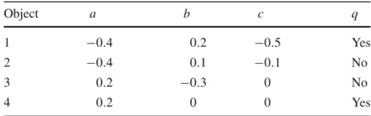
A simple worked example is presented here in order to illus-trate the MFNN algorithm. As summarised in Table1, it employs a dataset with 3 real-valued conditional attributes (a, bandc) and a single discrete-valued crisp decision attribute (q), as the training data. The two objects contained within Table2are employed as the test data for classification, which have the same numbers of conditional and decision attributes. Following the procedure of the MFNN algorithm, the first step is to calculate the similarities for all decision classes (∀x ∈ Dq where Dq stands for the domain of the decision

Table 1 Training data for the example

Object a b c q

1 −0.4 0.2 −0.5 Yes

2 −0.4 0.1 −0.1 No

3 0.2 −0.3 0 No

4 0.2 0 0 Yes

Table 2 Test data for the example

Object a b c q

t1 0.3 −0.3 0 No

t2 −0.3 0.3 −0.3 Yes

attribute, i.e., {yes,no}). For simplicity, the class member-ship is herein set to be crisp-valued. There are four objects that each belong to one of the two classes. Using the Ein-stein S-norm, Łukasiewicz T-norm (max(x + y −1,0)) (Borkowski 1970) and the following similarity metric [as defined inRadzikowska and Kerre(2002)]:

μRP(x,y)=Ta∈P{μRa(x,y)}, (3) the similarity of each test object can then be compared to all of the data objects in the training set. In (3),μRa(x,y)is the degree to which objects x andyare similar with regard to featureaand may be defined as (Jensen and Shen 2009):

μRa(x,y)=1−

|a(x)−a(y)| |amax−amin|.

(4) Note that for this simple exampleallneighbours are taken into consideration, i.e.,k= |U|.

For instance, consider the testing objectt1:

μR{P}(1,t1)=T(μR{a}(1,t1), μR{b}(1,t1), μR{c}(1,t1)) =0 μR{P}(2,t1)=T(μR{a}(2,t1), μR{b}(2,t1), μR{c}(2,t1)) =0 μR_{P_}(3,t1)=T(μR_{a_}(3,t1), μR_{b_}(3,t1), μR_{c_}(3,t1)) =0.86 μR{P}(4,t1)=T(μR{a}(4,t1), μR{b}(4,t1), μR{c}(4,t1)) =0.26 Then, for each class:

μR{P}(yes,t1)= μR{P}( 1,t1)+μR{P}(4,t1) 1+μR{P}(1,t1)∗μR{P}(4,t1) =(0+0.26)/(1+0∗0.26)=0.26 (5) μR{P}(no,t1)= μ R{P}(2,t1)+μR{P}(3,t1) 1+μR{P}(2,t1)∗μR{P}(3,t1) =(0+0.86)/(1+0∗0.86)=0.86 (6) Thus, the combination of similarities for the test objectt1 with respect to the class labelnois higher than that to the classyes. The algorithm will therefore classifyt1 as belong-ing to the classno. This procedure can then be repeated for

test objectt2 in exactly the same way, resulting int2 being classified as belonging to the classyes.

3 Relationship between MFNN and FRNN/VQNN

The flexible framework of the multi-functional neighbour algorithm allows it to cover many nearest-neighbour approaches as its special cases. This is demon-strated through the analysis of its relations with the state-of-the-art fuzzy-rough nearest-neighbour classification algo-rithms below.

3.1 Fuzzy-rough nearest-neighbour classification

The original fuzzy-rough nearest-neighbour (FRNN) algo-rithm was proposed inJensen and Cornelis(2011). In contrast to approaches such as fuzzy-rough ownership nearest neigh-bour (FRNN-O) (Sarkar 2007), FRNN employs the central rough set concepts in their fuzzified forms: fuzzy upper and lower approximations. These important concepts are used to determine the assignment of class membership to a given test object.

A fuzzy-rough set (Dubois and Prade 1992;Yao 1998) is defined by two fuzzy sets, obtained by extending the con-cepts of the upper and lower approximations in crisp rough sets (Pawlak 1991). In particular, the fuzzy upper and lower approximations of a certain objectyconcerning a fuzzy con-ceptX are defined as follows:

μRPX(y)= inf

x∈UI(μRP(x,y), μX(x)) (7)

μRPX(y)=sup

x∈U

T(μRP(x,y), μX(x)) (8) where I is a fuzzy implicator, T is a T-norm, μRP(x,y) is the fuzzy similarity defined in (3) and μX(x) is the

class membership function. More sophisticated mathemati-cal treatment of these can be found inJensen and Shen(2009) andRadzikowska and Kerre(2002).

The FRNN algorithm is outlined in Algorithm 2. As a extension of this method, vaguely quantified nearest neigh-bour (VQNN) has also been developed, as reported in Cornelis et al.(2007). This is achieved with the introduction of the lower and upper approximations of vaguely quantified rough sets (VQRS): μQu RPX(y)=Qu |RP(x,y)∩X| |RP(x,y)| =Qu ⎛ ⎜ ⎝ x∈U T(μRP(x,y), μX(x)) x_∈U μRP(x,y) ⎞ ⎟ ⎠, (9) μQl RPX(y)=Ql _| RP(x,y)∩X| |RP(x,y)| =Ql ⎛ ⎜ ⎝ x∈U T(μRP(x,y), μX(x)) x∈U μRP(x,y) ⎞ ⎟ ⎠. (10)

The pair(Qu,Ql)are fuzzy quantifiers (Cornelis et al. 2007),

with each element being an increasing[0,1] → [0,1] map-ping.

ALGORITHM 2: Fuzzy-rough nearest-neighbour algorithm

Input: ;

U, the training set;

C, the set of decision classes;

y, the object to be classified.

Output: Class, the classification result fory.

N ←get nearest neighbour(y,k);

τ←0,Class← ∅; for ∀X∈Cdo if(μRPX(y)+μRPX(y))/2≥τthen Class←X; τ←(μRPX(y)+μRPX(y))/2. end end

3.2 FRNN and VQNN as special instances of MFNN

Conceptually, MFNN is much simpler without the need of directly involving complicated mathematical definitions such as the above. However, its generality covers both FRNN and VQNN as its specific cases. Of the many methods for aggregating similarities,Gödel(Maximum)S-norm and the Addition operator are arguably amongst those which are most commonly used. By using these two aggregators, two particular implementations of MFNN can be devised, denot-ing them as MFNN_G (MFNN with Gödel S-norm) and MFNN_A (MFNN withAdditionoperator). If the fuzzy sim-ilarity defined in (3) and the crisp class membership function are employed to implement MFNN_G and MFNN_A, then, these two methods are, respectively, equivalent to FRNN and VQNN, in terms of classification outcomes. The proofs are given as follows.

Theorem 1 With the use of an identical fuzzy similarity met-ric, MFNN_G achieves the same classification accuracy as FRNN.

Proof Given a setUand a test objecty, consider using FRNN for classification first. Within the selected nearest neighbours, let M be the class that∃x∗ ∈ M, such thatμRP(x∗,y) = maxx∈U{μRP(x,y)}.For any a ∈ R, I(a,1) = 1 and

T(a,0)=0. Thus, due to the crisp membership function, for the decision conceptX = M, the lower and upper approxi-mations are reduced to:

μRPM(y)=inf inf x∈MI(μRP(x,y), μM(x)), inf x∈U−MI(μRP(x,y), μM(x)) = inf x_∈U−MI(μRP(x,y),0), (11) μRPM(y)=sup sup x∈M T(μRP(x,y), μM(x)), sup x∈U−M T(μRP(x,y), μM(x)) = sup x∈M T(μRP(x,y),1). (12) According to the properties of implicators andT-norms, for any giveny,I(x,y)is monotonically decreasing forx, and T(x,y)is monotonically increasing forx. In this case, (11) and (12) can be further simplified to:

μRPM(y)= I max x∈U−M{μRP(x,y)},0 , (13) μRPM(y)=T max x∈M{μRP(x,y)},1 =T(μRP(x∗,y),1). (14) Similarly, for the decision conceptX = L, where L is an arbitrary class different fromM, the following hold:

μRPL(y)= inf

x∈U−LI(μRP(x,y),0), (15)

μRPL(y)=sup

x∈L

T(μRP(x,y),1). (16) In the same way as (11) and (12), (15) and (16) are further reduced to: μRPL(y)=I max x∈U−L{μRP(x,y)},0 =I(μRP(x∗,y),0), (17) μRPL(y)=T max x∈L{μRP(x,y)},1 . (18) Since μRP(x∗,y)≥ max x∈U−M{μRP(x,y)} (19) μRP(x∗,y)≥max x_∈L{μRP(x,y)} (20)

according to the monotonic properties of implicators andT -norms, it can be derived that

μRPM(y)≥μRPL(y), (21) μRPM(y)≥μRPL(y). (22) Therefore, μRPM(y)+μRPM(y) 2 ≥ μRPL(y)+μRPL(y) 2 . (23)

Because of the arbitrariness of classL, following the method of FRNN,ywill be classified into classM.

Now, consider the use of MFNN_G. Given the same assumptions and parameters as assumed above, because MFNN_G is implemented by the same fuzzy similarity met-ric as FRNN, these two methods will share the identical nearest neighbours as well. And forx∗∈ M, it can be derived that A x∈MμRP(x,y)μM(x)=x∈AMμRP(x,y)·1 =max x∈M{μRP(x,y)} =μRP(x∗,y) =max x∈U{μRP(x,y)} ≥max x∈L{μRP(x,y)} = A x∈LμRP(x,y)μL(x) (24)

Because of the arbitrariness of classL, following the method of MFNN, ywill be classified into class M. Therefore, the classification outcome of MFNN_G is identical to that of

FRNN.

Theorem 2 With the use of an identical fuzzy similarity met-ric, MFNN_A achieves the same classification accuracy as VQNN.

Proof Given a setUand a test objecty, Within the selected nearest neighbours, letMbe the class that_x∈MμRP(x,y) =max

X∈C{

x∈XμRP(x,y)}, whereCdenotes the set of deci-sion classes.

According to the definition of VQNN, for the decision concept X=M, the lower and upper approximations are

μQu RPM(y)=Qu ⎛ ⎜ ⎝ x∈U T(μRP(x,y), μM(x)) x∈U μRP(x,y) ⎞ ⎟ ⎠ =Qu ⎛ ⎜ ⎝ x∈M T(μRP(x,y), μM(x)) x∈U μRP(x,y) + x∈/M T(μRP(x,y), μM(x)) x_∈U μRP(x,y) ⎞ ⎟ ⎠ (25)

μQl RPM(y)=Ql ⎛ ⎜ ⎝ x∈U T(μRP(x,y), μM(x)) x∈U μRP(x,y) ⎞ ⎟ ⎠ =Ql ⎛ ⎜ ⎝ x∈M T(μRP(x,y), μM(x)) x∈U μRP(x,y) + x∈/M T(μRP(x,y), μM(x)) x∈U μRP(x,y) ⎞ ⎟ ⎠ (26)

BecauseT(a,0)=0,T(a,1)=aand the class membership is crisp-valued, (25) and (26) can be simplified as

μQu RPM(y)=Qu ⎛ ⎜ ⎝ x∈M μRP(x,y) x∈U μRP(x,y) ⎞ ⎟ ⎠ (27) μQl RPM(y)=Ql ⎛ ⎜ ⎝ x∈M μRP(x,y) x∈U μRP(x,y) ⎞ ⎟ ⎠. (28)

Similarly, for a distinct decisionX =L, the lower and upper approximation can be, respectively, denoted by

μQu RPL(y)=Qu ⎛ ⎜ ⎝ x∈L μRP(x,y) x∈U μRP(x,y) ⎞ ⎟ ⎠ (29) μQl RPL(y)=Ql ⎛ ⎜ ⎝ x_∈L μRP(x,y) x∈U μRP(x,y) ⎞ ⎟ ⎠. (30)

Following the definition of VQNN, the fuzzy qualifier in VQNN is an increasing[0,1] → [0,1]relation. In this case, because x∈M μRP(x,y)≥ x∈L μRP(x,y), (31)

it can be established that

μQu RPM(y)≥μ Qu RPL(y) (32) μQl RPM(y)≥μ Ql RPL(y), (33) Then, obviously, μQu RPM(y)+μ Ql RPM(y) 2 ≥ μQu RPL(y)+μ Ql RPL(y) 2 (34)

This concludes thatywill always be classified into ClassM.

For MFNN_A, from the same assumptions and parameters which are used above, due to the identical nearest neighbours to those of VQNN, it can be derived that

A x∈MμRP(x,y)μM(x)=x∈AMμRP(x,y)× 1 = x∈M μRP(x,y) =max X∈C x∈X μRP(x,y) ≥ x∈L μRP(x,y) = A x_∈LμRP(x,y)μL(x) (35)

Because of the arbitrariness of classL, according to the defi-nition of MFNN,ywill be classified into classM. Therefore, the classification outcome of MFNN_A is the same as that

of VQNN.

It is noteworthy that, implemented by above configu-ration, MFNN_G and MFNN_A, are equivalent to FRNN and VQNN, respectively, only in the sense that they can achieve the same classification outcome and hence the same classification accuracy. However, the actual underlying pre-dicted probabilities and models of MFNN_G/MFNN_A and FRNN/VQNN are different. Therefore, for other classifica-tion performance indicators, such as root-mean-squared error (RMSE), which are determined by the numerical predicted probabilities, the equivalent relationships between MFNN_G /MFNN_A and FRNN/VQNN may not hold.

4 Popular nearest-neighbour methods as special

cases of MFNN

To further demonstrate the generality of MFNN, this sec-tion discusses the relasec-tionship between MFNN andknearest neighbour and that between MFNN and fuzzy nearest neigh-bour.

4.1 K nearest neighbour and MFNN

As introduced previously, the k nearest-neighbour (kNN) classifier (Cover and Hart 1967) assigns a test object to the class that is best represented amongst its k nearest neigh-bours.

In implementing MFNN, in addition to the use of the crisp class membership, the cardinality measure can be employed to perform the aggregation. More specifically, the aggrega-tion of the similarities with respect to each class X for the given setNofknearest neighbours can be defined as:

A

x_∈NμRP(x,y)μX(x)=x_∈NA_∩XμRP(x,y)

=

x_∈N_∩X

f(μRP(x,y)), (36) where the function f(·) ≡ 1. In so doing, the aggregation of the similarities and the class membership for each class within theknearest neighbours is the number of such ele-ments that are nearest to the test object. Therefore, the test object will be classified into the class which is the most com-mon acom-mongst itsknearest neighbours by MFNN. As such, MFNN becomeskNN if (the opposite of) the Euclidean dis-tance in (1) is used to measure the similarity as it is used to measure the closeness inkNN.

4.2 Fuzzy nearest neighbour and MFNN

In fuzzy nearest neighbour (FNN) (Keller et al. 1985), thek nearest neighbours of the test instance are determined first. Then, the test instance is assigned to the class for which the decision qualifier (2) is maximal.

Note that the similarity relation in MFNN can be config-ured such that

μRP(x,y)=d(x,y)− 2

m−1, ₍₃₇₎

which is indeed a valid similarity metric. Note also that by setting the aggregator as the weighted summation, with the weights uniformly set to 1

x∈NμR P(x,y), the decision indica-tor of MFNN becomes: A x∈NμRP(x,y)μX(x) = ⎛ ⎜ ⎝ 1 x∈N μRP(x,y) ⎞ ⎟ ⎠ x∈N μRP(x,y)μX(x), (38)

whereμX(x)is the same class membership used in FNN as

well. In so doing, FNN and MFNN will have the identical classification results. For FRNN-O (Sarkar 2007), similar conclusions also hold. The analyses regarding both cases are parallel to the above and therefore, omitted here.

5 Experimental evaluation

This section presents a systematic evaluation of MFNN experimentally. The results and discussions are divided into four different parts, after an introduction to the experimen-tal set-up. The first part investigates the influence of the number of nearest neighbours on the MFNN algorithm and how this may affect classification performance. The second

compares MFNN with five other nearest-neighbour meth-ods in term of classification accuracy. It also demonstrates empirically how MFNN may be equivalent to the fuzzy-rough set-based FRNN and VQNN approaches, supporting the earlier formal proofs. The third and fourth parts provide a comparative investigation of the performance of several ver-sions of the MFNN algorithm against four state-of-the-art classifier learners. Once again, these comparisons are made with regard to the classification accuracy.

5.1 Experimental set-up

Sixteen benchmark datasets obtained fromArmanino et al. (1989) andBlake and Merz(1998) are used for the experi-mental evaluation. These datasets contain between 120 and 6435 objects with numbers of features ranging from 6 to 649, as summarised in Table3.

For the present study, MFNN employs the popular relation of (4) and the Kleene-DienesT-norm (Dienes 1949;Kleene 1952) to measure the fuzzy similarity as per (3) in the follow-ing experiments. Whilst this does not allow the opportunity to fine-tune individual MFNN methods, it ensures that methods are compared on equal footing. For simplicity, in the follow-ing experiments, the class membership functions utilised in MFNN are consistently set to be crisp-valued.

Stratified 10 × 10-fold cross-validation (10-FCV) is employed throughout the experimentation. In 10-FCV, an original dataset is partitioned into 10 subsets of data objects. Of these 10 subsets, a single subset is retained as the test-ing data for the classifier, and the remaintest-ing 9 subsets are used for training. The cross-validation process is repeated

Table 3 Datasets used for evaluation

Dataset Objects Attributes

Cleveland 297 13 Ecoli 336 7 Glass 214 9 Handwritten 1593 256 Heart 270 13 Liver 345 6 Multifeat 2000 649 Olitos 120 25 Page-block 5473 10 Satellite 6435 36 Sonar 208 60 Water 2 390 38 Water 3 390 38 Waveform 5000 40 Wine 178 14 Wisconsin 683 9

for 10 times. The 10 sets of results are then averaged to pro-duce a single classifier estimation. The advantage of 10-FCV over random subsampling is that all objects are used for both training and testing, and each object is used for testing only once per fold. The stratification of the data prior to its division into folds ensures that each class label (as far as possible) has equal representation in all folds, thereby helping to alleviate bias/variance problems (Bengio and Grandvalet 2005).

A paired t-test with a significance level of 0.05 is employed to provide statistical analysis of the resulting clas-sification accuracy. This is done in order to ensure that results are not discovered by chance. The baseline references for the tests are the classification accuracy obtained by MFNN. The results on statistical significance are summarised in the final line of each table, showing a count of the number of statis-tically better (v), equivalent ( ) or worse (*) cases for each method in comparison to MFNN. For example, in Table4, (2/8/6) in the FNN column indicates that MFNN_G performs better than this method on 6 datasets, equivalently to it on 8 datasets, and worse than it in just 2 datasets.

5.2 Influence of number of neighbours

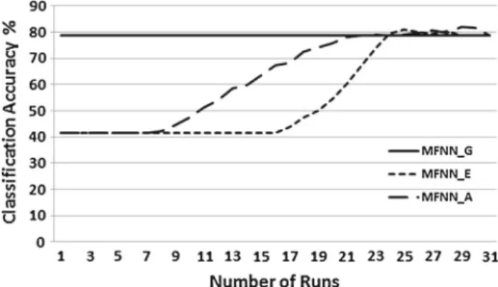
As mentioned previously, when using theGödeloperator and crisp class membership, the classification accuracy of MFNN is not affected by the selection of the value ofk. This is not generally the case when other operators are employed. In order to demonstrate this empirically, the impact of differ-ent values ofk is investigated for MFNN on two datasets, heartandolitos. TheEinsteinandAdditionoperators as well as theGödel S-norm are used to implement MFNN, with the resulting classifiers denoted as MFNN_E, MFNN_A and MFNN_G, respectively. For the investigation described here, kis initially set to|U|(the total number of the objects in the dataset) and then decremented by 1/30 of|U|each time, with an extra round for the case whenk =1. This results in 31 runs for each of the two datasets. For each value ofk, 10× 10-fold cross-validation is performed. The results for these two datasets are shown in Figs.1and2.

It can be seen that MFNN_G is unaffected by the choice of k. However, MFNN_E and MFNN_A initially exhibit improvement in classification performance, followed by a degradation for both datasets as the value ofk decreases. Therefore, the choice of value forkis an important considera-tion when using an aggregator other than theGödeloperator. Careful off-line selection of an appropriatek is necessary before MFNN is applied (unless MFNN_G is to be used). This conforms to the general findings in thekNN literature.

5.3 Comparison with other nearest neighbour methods

This section presents a comparison of MFNN with other five nearest-neighbour classification methods:k nearest

neigh-Fig. 1 Classification accuracy of three MFNNs (Gödel,Einstein, Addi-tion) with respect to differentkvalues for theheartdataset

Fig. 2 Classification accuracy of three MFNNs (Gödel,Einstein, Addi-tion) with respect to differentkvalues for theolitosdataset

bour (kNN) (Cover and Hart 1967), fuzzy nearest neighbour (FNN) (Keller et al. 1985), fuzzy-rough ownership nearest neighbour (FRNN-O) (Sarkar 2007), fuzzy-rough nearest neighbour (FRNN) (Jensen and Cornelis 2011) and vaguely quantified nearest neighbour (VQNN) (Cornelis et al. 2007). In order to provide a fair comparison, all of the results are generated with the value ofkset to 10 when implementing MFNN_A, VQNN, FNN, FRNN-O andkNN.

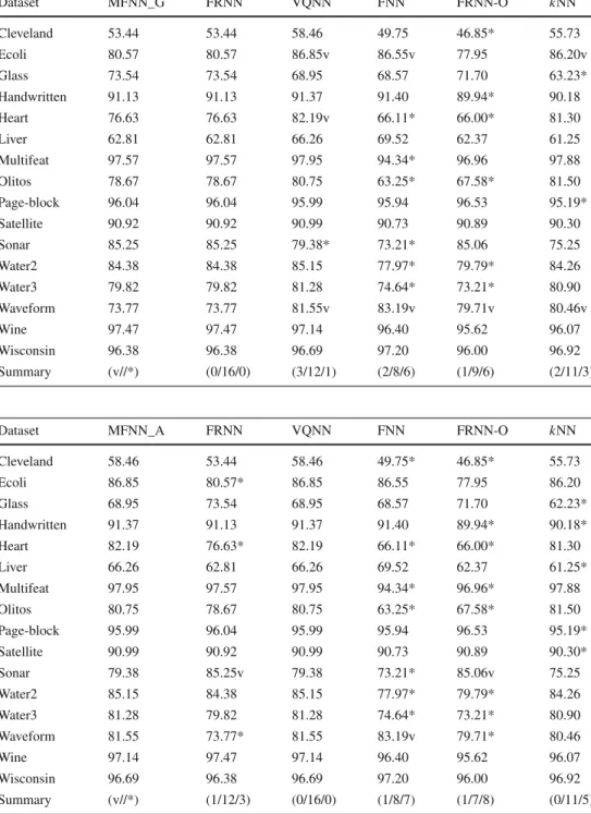
Tables 4 and 5 show that as expected, for all datasets, MFNN_G and MFNN_A offer identical classification accu-racies to those of FRNN and VQNN, respectively. When compared to FNN, FRNN-O andkNN, different implemen-tations of MFNN generally return statistically better or equal results, especially for thecleveland,heart,olitos,water2, and water3datasets. This is shown in these two tables and also in Table6(for MFNN_E). There are very occasional cases where MFNN methods perform less well. In particular, for thewaveformdataset, the MFNN classifiers fail to perform so well as FNN, but these few results do not reflect the general trend in which MFNN methods outperform the rest.

Comparing the three MFNN classifiers themselves, MFNN_A statistically achieves the best performance, with an exception for thesonardataset. MFNN_E also performs

Table 4 Classification accuracy: MFNN_G versus others Dataset MFNN_G FRNN VQNN FNN FRNN-O kNN Cleveland 53.44 53.44 58.46 49.75 46.85* 55.73 Ecoli 80.57 80.57 86.85v 86.55v 77.95 86.20v Glass 73.54 73.54 68.95 68.57 71.70 63.23* Handwritten 91.13 91.13 91.37 91.40 89.94* 90.18 Heart 76.63 76.63 82.19v 66.11* 66.00* 81.30 Liver 62.81 62.81 66.26 69.52 62.37 61.25 Multifeat 97.57 97.57 97.95 94.34* 96.96 97.88 Olitos 78.67 78.67 80.75 63.25* 67.58* 81.50 Page-block 96.04 96.04 95.99 95.94 96.53 95.19* Satellite 90.92 90.92 90.99 90.73 90.89 90.30 Sonar 85.25 85.25 79.38* 73.21* 85.06 75.25 Water2 84.38 84.38 85.15 77.97* 79.79* 84.26 Water3 79.82 79.82 81.28 74.64* 73.21* 80.90 Waveform 73.77 73.77 81.55v 83.19v 79.71v 80.46v Wine 97.47 97.47 97.14 96.40 95.62 96.07 Wisconsin 96.38 96.38 96.69 97.20 96.00 96.92 Summary (v//*) (0/16/0) (3/12/1) (2/8/6) (1/9/6) (2/11/3) Table 5 Classification accuracy: MFNN_A versus others

Dataset MFNN_A FRNN VQNN FNN FRNN-O kNN

Cleveland 58.46 53.44 58.46 49.75* 46.85* 55.73 Ecoli 86.85 80.57* 86.85 86.55 77.95 86.20 Glass 68.95 73.54 68.95 68.57 71.70 62.23* Handwritten 91.37 91.13 91.37 91.40 89.94* 90.18* Heart 82.19 76.63* 82.19 66.11* 66.00* 81.30 Liver 66.26 62.81 66.26 69.52 62.37 61.25* Multifeat 97.95 97.57 97.95 94.34* 96.96* 97.88 Olitos 80.75 78.67 80.75 63.25* 67.58* 81.50 Page-block 95.99 96.04 95.99 95.94 96.53 95.19* Satellite 90.99 90.92 90.99 90.73 90.89 90.30* Sonar 79.38 85.25v 79.38 73.21* 85.06v 75.25 Water2 85.15 84.38 85.15 77.97* 79.79* 84.26 Water3 81.28 79.82 81.28 74.64* 73.21* 80.90 Waveform 81.55 73.77* 81.55 83.19v 79.71* 80.46 Wine 97.14 97.47 97.14 96.40 95.62 96.07 Wisconsin 96.69 96.38 96.69 97.20 96.00 96.92 Summary (v//*) (1/12/3) (0/16/0) (1/8/7) (1/7/8) (0/11/5)

slightly better than MFNN_G. This is due to the fact that the classification results gained by MFNN_G only rely on one sample. In this case, MFNN_G is sensitive to noisy data, whilst MFNN_A is significantly more robust in the presence of noisy data.

Overall, considering all the experimental results, this method outperforms all of the existing methods. This makes MFNN_A a potentially good candidate for many classifica-tion tasks.

5.4 Comparison with the state of the art: use of different aggregators

This section experimentally compares MFNN with several leading classifier learners that represent a cross section of the most popular approaches. For completeness, a brief summary of these methods is provided below.

– PART (Witten and Frank 1998, 2000) generates rules by means of repeatedly creating partial decision trees

Table 6 Classification accuracy: MFNN_E versus others

Dataset MFNN_E FRNN VQNN FNN FRNN-O kNN

Cleveland 53.64 53.44 58.46 49.75 46.85* 55.73 Ecoli 81.93 80.57* 86.85v 86.55v 77.95 86.20v Glass 74.29 73.54 68.95 68.57 71.70 63.23* Handwritten 91.20 91.13 91.37 91.40 89.94* 90.18 Heart 76.70 76.63 82.19v 66.11* 66.00* 81.30 Liver 63.07 62.81 66.26 69.52 62.37 61.25 Multifeat 97.59 97.57 97.95 94.34* 96.96 97.88 Olitos 78.83 78.67 80.75 63.25* 67.58* 81.50 Page-block 96.18 96.04 95.99 95.94 96.53 95.19* Satellite 91.52 90.92* 90.99 90.73* 90.89* 90.30* Sonar 85.35 85.25 79.38* 73.21* 85.06 75.25* Water2 85.21 84.38 85.15 77.97* 79.79* 84.26 Water3 80.77 79.82 81.28 74.64* 73.21* 80.90 Waveform 74.97 73.77* 81.55v 83.19v 79.71v 80.46v Wine 97.47 97.47 97.14 96.40 95.62 96.07 Wisconsin 96.38 96.38 96.69 97.20 96.00 96.92 Summary (v//*) (0/13/3) (3/12/1) (2/7/7) (1/8/7) (2/10/4)

from the data. The algorithm adopts a divide-and-conquer strategy such that it removes instances already covered by the current ruleset during the learning processing. Essen-tially, a rule is created by building a pruned tree for the current set of instances; the branch leading to a leaf with the highest coverage is promoted to a classification rule. In this paper, this method is empirically learned with a confident factor of 0.25.

– J48 is based on ID3 (Quinlan 1993) and creates deci-sion trees by choosing the most informative features and recursively partitioning a training data table into subta-bles based on the values of such features. Each node in the tree represents a feature, with the subsequent nodes branching from the possible values of this node accord-ing to the current subtable. Partitionaccord-ing stops when all data items in the subtable have the same classification. A leaf node is then created to represent this classifica-tion. In this paper, J48 is set with the pruning confidence thresholdC =0.25.

– SMO (Smola and Schölkopf 1998) is an algorithm for efficiently solving optimisation problems which arise during the training of a support vector machine (Cortes and Vapnik 1995). It breaks optimisation problems into a series of smallest possible subproblems, which are then resolved analytically. In this paper, SMO is set with C = 1, tolerance L = 0.001, round-off error=10−12, data running on normalised and polynomial kernel. – NB (Naive Bayes) (John and Langley 1995) is a simple

probabilistic classifier, directly applying Bayes’ theo-rem (Papoulis 1984) with strong (naive) independence assumptions. Depending on the precise nature of the

Table 7 Classification accuracy of MFNN_G

Dataset MFNN_G PART J48 SMO NB

Cleveland 53.44 52.44 53.39 58.31 56.06 Ecoli 80.57 81.79 82.83 83.48 85.50v Glass 73.54 69.12 68.08 57.77* 47.70* Handwritten 91.13 79.34* 76.13* 93.58v 86.19* Heart 76.63 77.33 78.15 83.89v 83.59v Liver 62.81 65.25 65.84 57.98 54.89 Multifeat 97.57 94.68* 94.62* 98.39v 95.27* Olitos 78.67 67.00* 65.75* 87.92v 78.50 Page-block 96.04 96.93v 96.99v 92.84* 90.01* Satellite 90.92 86.63* 86.41* 86.78* 79.59* Sonar 85.25 77.40* 73.61* 76.60* 67.71* Water2 84.38 83.85 83.18 83.64 69.72* Water3 79.82 82.72 81.59 87.21v 85.49v Waveform 73.77 77.62v 75.25 86.48v 80.01v Wine 97.47 92.24* 93.37 98.70 97.46 Wisconsin 96.38 95.68 95.44 97.01 96.34 Summary (v//*) (2/8/6) (1/10/5) (6/6/4) (4/5/7)

probability model used, naive Bayesian classifiers can be trained very efficiently in a supervised learning setting. The learning only requires a small amount of training data to estimate the parameters (means and variances of the variables) necessary for classification.

The results are listed in Tables7,8and9, together with a statistical comparison between each method and MFNN_G, MFNN_E and MFNN_A, respectively.

Table 8 Classification accuracy of MFNN_E

Dataset MFNN_E PART J48 SMO NB

Cleveland 53.64 52.44 53.39 58.31 56.06 Ecoli 81.93 81.79 82.83 83.48 85.50 Glass 74.29 69.12 68.08 57.77* 47.70* Handwritten 91.20 79.34* 76.13* 93.58v 86.19* Heart 76.70 77.33 78.15 83.89v 83.59v Liver 63.07 65.25 65.84 57.98 54.89 Multifeat 97.59 94.68* 94.62* 98.39v 95.27* Olitos 78.83 67.00* 65.75* 87.92v 78.50 Page-block 96.18 96.93v 96.99v 92.84* 90.01* Satellite 91.52 86.63* 86.41* 86.78* 79.59* Sonar 85.35 77.40* 73.61* 76.60* 67.71* Water2 85.21 83.85 83.18 83.64 69.72* Water3 80.77 82.72 81.59 87.21v 85.49v Waveform 74.97 77.62v 75.25 86.48v 80.01v Wine 97.47 92.24* 93.37 98.70 97.46 Wisconsin 96.38 95.68 95.44 97.01 96.34 Summary (v//*) (2/8/6) (1/10/5) (6/6/4) (3/6/7)

Table 9 Classification accuracy of MFNN_A

Dataset MFNN_A PART J48 SMO NB

Cleveland 58.46 52.44* 53.39 58.31 56.06 Ecoli 86.85 81.79* 82.83* 83.48 85.50 Glass 68.95 69.12 68.08 57.77* 47.70* Handwritten 91.37 79.34* 76.13* 93.58v 86.19* Heart 82.19 77.33 78.15 83.89 83.59 Liver 66.26 65.25 65.84 57.98* 54.89* Multifeat 97.95 94.68* 94.62* 98.39 95.27* Olitos 80.75 67.00* 65.75* 87.92v 78.50 Page-block 95.99 96.93v 96.99v 92.84* 90.01* Satellite 90.99 86.63* 86.41* 86.78* 79.59* Sonar 79.38 77.40 73.61 76.60 67.71* Water2 85.15 83.85 83.18 83.64 69.72* Water3 81.28 82.72 81.59 87.21v 85.49v Waveform 81.55 77.62* 75.25* 86.48v 80.01 Wine 97.14 92.24* 93.37 98.70 97.46 Wisconsin 96.69 95.68 95.44 97.01 96.34 Summary (v//*) (1/7/8) (1/9/6) (4/8/4) (1/7/8)

It can be seen from these results that in general, all three implemented MFNN methods perform well. In par-ticular, even considering MFNN_G, the least performer amongst the three, for theglass,satellite,sonar, andwater 2 datasets, it achieves statistically better classification perfor-mance against all the other types of classifier. Only for the ecoliandwaveformdatasets, MFNN_G does not perform so well as it does on the other datasets.

Amongst the three MFNN implementations, MFNN_A is again the best performer. It is able to generally improve the classification accuracies achievable by both MFNN_G and MFNN_E, for the cleveland, ecoli,heart, liver,waveform datasets. However, from a statistical perspective, its perfor-mance is similar to the other two overall. Nevertheless, in terms of accuracy, MFNN_A is statistically better than PART, J48 and NB, respectively, for 8, 6 and 8 datasets, with an equal statistical performance to that of SMO.

5.5 Comparison with the state of the art: use of different similarity metrics

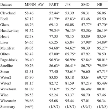
It was mentioned previously that the MFNN approach offers significant flexibility as it allows the use of different simi-larity metrics and aggregation operators. To provide a more comprehensive view of the performance of MFNN, this sec-tion investigates the effect of employing different similarity metrics. In particular, kernel-based fuzzy similarity met-rics are employed in this section (Qu et al. 2015). Such similarity metrics are induced by the stationary kernel func-tions and robustness in statistics. Specifically, as the overall best, MFNN_A is modified to use either the wave kernel function or the rational quadratic kernel function. The resul-tant classifiers are denoted by MFNN_AW and MFNN_AR, respectively.

As demonstrated in Tables10and11, the classification accuracies achieved by MFNN_AW and MFNN_AR further improve over those achieved by MFNN_A for a number of datasets. Statistically, it is shown that MFNN_AW generally

Table 10 Classification accuracy of MFNN_AW

Dataset MFNN_AW PART J48 SMO NB

Cleveland 58.46 52.44* 53.39 58.31 56.06 Ecoli 87.12 81.79* 82.83* 83.48 85.50 Glass 66.76 69.12 68.08 57.77* 47.70* Handwritten 91.32 79.34* 76.13* 93.58v 86.19* Heart 82.78 77.33 78.15 83.89 83.59 Liver 64.65 65.25 65.84 57.98* 54.89* Multifeat 98.05 94.68* 94.62* 98.39 95.27* Olitos 82.42 67.00* 65.75* 87.92 78.50 Page-block 96.40 96.93v 96.99v 92.84* 90.01* Satellite 90.76 86.63* 86.41* 86.78* 79.59* Sonar 81.31 77.40 73.61* 76.60 67.71* Water2 85.90 83.85 83.18 83.64 69.72* Water3 81.15 82.72 81.59 87.21v 85.49v Waveform 81.09 77.62* 75.25* 86.48v 80.01 Wine 96.53 92.24 93.37 98.70 97.46 Wisconsin 96.66 95.68 95.44 97.01 96.34 Summary (v//*) (1/8/7) (1/8/7) (3/9/4) (1/7/8)

Table 11 Classification accuracy of MFNN_AR

Dataset MFNN_AR PART J48 SMO NB

Cleveland 57.21 52.44 53.39 58.31 56.06 Ecoli 87.68 81.79* 82.83* 83.48* 85.50 Glass 74.98 69.12 68.08 57.77* 47.70* Handwritten 91.29 79.34* 76.13* 93.58v 86.19* Heart 81.93 77.33 78.15 83.89 83.59 Liver 64.88 65.25 65.84 57.98* 54.89* Multifeat 97.75 94.68* 94.62* 98.39v 95.27* Olitos 80.67 67.00* 65.75* 87.92v 78.50 Page-block 96.09 96.93v 96.99v 92.84* 90.01* Satellite 90.01 86.63* 86.41* 86.78* 79.59* Sonar 77.02 77.40 73.61 76.60 67.71* Water2 85.03 83.85 83.18 83.64 69.72* Water3 80.82 82.72 81.59 87.21v 85.49v Waveform 80.14 77.62* 75.25* 86.48v 80.01 Wine 95.97 92.24 93.37 98.70 97.46 Wisconsin 96.35 95.68 95.44 97.01 96.34 Summary (v//*) (1/9/6) (1/9/6) (5/6/5) (1/7/8)

outperforms the other approaches (particularly for theolitos dataset). MFNN_AR also outperforms all the other classifiers with the exception of SMO (to which MFNN_AR obtains a comparable and statistically equal performance). Note that for theglassdataset, MFNN_AR achieves a very significant improvement in accuracy.

In summary, examining all of the results obtained, it has been experimentally shown that when a kernel-based fuzzy similarity metric is employed, MFNN offers a better and more robust performance than the other classifiers.

6 Conclusion

This paper has presented a multi-functional nearest-neighbour approach (MFNN). In this work, the combina-tion of fuzzy similarities and class memberships may be performed using different aggregators. Such an aggregated similarity measure is then employed as the decision qualifier for the process of decision-making in classification.

The wide and variable choice of the aggregators and fuzzy similarity metrics ensures that the proposed approach has a high flexibility and is of significant generality. For exam-ple, using appropriate similarity relations, aggregators and class membership functions, MFNN can perform the tasks of classicalkNN and FNN. Such construction helps to ensure that the resulting MFNN is adaptive in dealing with differ-ent classification problems given a wide range of choices. Furthermore, using theGödel S-norm andAddition opera-tor, the resulting specific MFNN implementations (with crisp

membership) have the ability to achieve the same classifi-cation accuracy as two advanced fuzzy-rough set methods: fuzzy-rough nearest neighbour (FRNN) and vaguely quan-tified nearest neighbours (VQNN). That is, both traditional nearest-neighbour methods and advanced fuzzy-rough-based classifiers can be seen as special cases of MFNN. This obser-vation indicates that the MFNN algorithm grants a flexible framework to the existing nearest-neighbour classification methods. These results are proven by theoretical analysis, supported with empirical results.

To demonstrate the efficacy of the MFNN approach, systematic experiments have been carried out from the perspective of classification accuracy. The results of the experimental evaluation have been very promising. They demonstrate that implemented with specific aggregators, par-ticularly whilst employing theAdditionoperator, MFNN can generally outperform a range of state-of-the-art learning clas-sifiers in terms of these performance indicators.

Topics for further research include a more comprehen-sive study of how the proposed approach would perform in regression or other prediction tasks, where the decision vari-ables are not crisp. Also, recently, a proposal has been made to develop techniques for efficient information aggregation and unsupervised feature selection, which exploits the con-cept of nearest-neighbour-based data reliability (Boongoen and Shen 2010;Boongoen et al. 2011). An investigation into how the present work could be used to perform such tasks or perhaps (semi-)supervised feature selection (Jensen and Shen 2008) remains active research.

Acknowledgements This work was jointly supported by the National Natural Science Foundation of China (No. 61502068) and the China Postdoctoral Science Foundation (Nos. 2013M541213 and 2015T80239). The authors would also like to thank the financial support provided by Aberystwyth University and the colleagues in the Advanced Reasoning Group with the Department of Computer Science, Institute of Mathematics, Physics and Computer Science at Aberystwyth Uni-versity, UK.

Compliance with ethical standards

Conflict of interest The authors declare that they have no conflict of interest.

Open Access This article is distributed under the terms of the Creative Commons Attribution 4.0 International License (http://creativecomm ons.org/licenses/by/4.0/), which permits unrestricted use, distribution, and reproduction in any medium, provided you give appropriate credit to the original author(s) and the source, provide a link to the Creative Commons license, and indicate if changes were made.

References

Armanino C, Leardia R, Lanteria S, Modi G (1989) Chemometric anal-ysis of tuscan olive oils. Chemom Intell Lab Syst 5:343–354 Baets BD, Mesiar R (1998) T-partitions. Fuzzy Sets Syst 97:211–223

Baets BD, Mesiar R (2002) Metrics and T-equalities. J Math Anal Appl 267:531–547

Bengio Y, Grandvalet Y (2005) Bias in estimating the variance ofK -fold cross-validation. In: Duchesne P, RÉMillard B (eds) Statistical modeling and analysis for complex data problems. Springer, Bas-ton, pp 75–95

Blake CL, Merz CJ (1998) UCI repository of machine learning databases. University of California, School of Information and Computer Sciences, Irvine

Boongoen T, Shang C, Iam-On N, Shen Q (2011) Nearest-neighbor guided evaluation of data reliability and its applications. IEEE Trans Syst Man Cybern Part B Cybern 41:1705–1714

Borkowski L (ed) (1970) Selected works by Jan Łukasiewicz. North-Holland Publishing Co., Amsterdam

Boongoen T, Shen Q (2010) Nearest-neighbor guided evaluation of data reliability and its applications. IEEE Trans Syst Man Cybern Part B Cybern 40:1622–1633

Breiman L, Friedman JH, Olshen RA, Stone CJ (1984) Classification and regression trees. Wadsworth & Brooks, Monterey, CA Cornelis C, Cock MD, Radzikowska A (2007) Vaguely quantified rough

sets. In: Lecture notes in artificial intelligence, vol 4482. pp 87–94 Cortes C, Vapnik V (1995) Support-vector networks. Mach Learn

20:273–297

Cover T, Hart P (1967) Nearest neighbor pattern classification. IEEE Trans. Inf. Theory 13:21–27

Daelemans W, den Bosch AV (2005) Memory-based language process-ing. Cambridge University Press, Cambridge

Das M, Chakraborty MK, Ghoshal TK (1998) Fuzzy tolerance relation, fuzzy tolerance space and basis. Fuzzy Sets Syst 97:361–369 Dienes SP (1949) On an implication function in many-valued systems

of logic. J Symb Logic 14:95–97

Dubois D, Prade H (1992) Putting rough sets and fuzzy sets together. Intelligent decision support, Springer, Dordrecht, pp 203–232 Duda RO, Hart PE, Stork DG (2001) Pattern classification, 2nd edn.

Wiley, Hoboken

Jensen R, Cornelis C (2011) A new approach to fuzzy-rough near-est neighbour classification. In: Transactions on rough sets XIII, LNCS, vol 6499. pp 56–72

Jensen R, Shen Q (2008) Computational intelligence and feature selec-tion: rough and fuzzy approaches. Wiley, Indianapolis

Jensen R, Shen Q (2009) New approaches to fuzzy-rough feature selec-tion. IEEE Trans Fuzzy Syst 17:824–838

John GH, Langley P (1995) Estimating continuous distributions in Bayesian classifiers. In: Eleventh conference on uncertainty in arti-ficial intelligence, pp 338–345

Keller JM, Gray MR, Givens JA (1985) A fuzzy k-nearest neighbor algorithm. IEEE Trans Syst Man Cybern 15:580–585

Kleene SC (1952) Introduction to metamathematics. Van Nostrand, New York

Kolmogorov AN (1950) Foundations of the theory of probability. Chelsea Publishing Co., Chelsea

Papoulis A (1984) Probability, random variables, and stochastic pro-cesses, 2nd edn. McGraw-Hill, New York

Pawlak Z (1991) Rough sets: theoretical aspects of reasoning about data. Kluwer Academic Publishing, Norwell

Qu Y, Shang C, Shen Q, Mac Parthaláin N, Wu W (2015) Kernel-based fuzzy-rough nearest-neighbour classification for mammographic risk analysis. Int J Fuzzy Syst 17:471–483

Quinlan JR (1993) C4.5: Programs for machine learning., The Morgan Kaufmann series in machine learningMorgan Kaufmann, Burling-ton

Radzikowska AM, Kerre EE (2002) A comparative study of fuzzy rough sets. Fuzzy Sets Syst 126:137–155

Sarkar M (2007) Fuzzy-rough nearest neighbors algorithm. Fuzzy Sets Syst 158:2123–2152

Smola AJ, Schölkopf B (1998) A tutorial on support vector regression. Neuro-COLT2 Technical Report Series, NC2-TR-1998-030 Witten IH, Frank E (1998) Generating accurate rule sets without global

optimisation. In: Proceedings of the 15th international conference on machine learning, San Francisco. Morgan Kaufmann Witten IH, Frank E (2000) Data mining: practical machine learning

tools with Java implementations. Morgan Kaufmann, Burlington Yager RR (1988) On ordered weighted averaging aggregation operators

in multi-criteria decision making. IEEE Trans Syst Man Cybern 18:183–190

Yao YY (1998) A comparative study of fuzzy sets and rough sets. Inf Sci 109:227–242