A note on uniform consistency of monotone function estimators

econstor

www.econstor.eu

Nutzungsbedingungen:

Die ZBW räumt Ihnen als Nutzerin/Nutzer das unentgeltliche, räumlich unbeschränkte und zeitlich auf die Dauer des Schutzrechts beschränkte einfache Recht ein, das ausgewählte Werk im Rahmen der unter

→ http://www.econstor.eu/dspace/Nutzungsbedingungen nachzulesenden vollständigen Nutzungsbedingungen zu vervielfältigen, mit denen die Nutzerin/der Nutzer sich durch die erste Nutzung einverstanden erklärt.

Terms of use:

The ZBW grants you, the user, the non-exclusive right to use the selected work free of charge, territorially unrestricted and within the time limit of the term of the property rights according to the terms specified at

→ http://www.econstor.eu/dspace/Nutzungsbedingungen By the first use of the selected work the user agrees and declares to comply with these terms of use.

zbw

Neumeyer, Natalie

Working Paper

A note on uniform consistency of

monotone function estimators

Technical Report / Universität Dortmund, SFB 475 Komplexitätsreduktion in Multivariaten Datenstrukturen, No. 2005,35

Provided in cooperation with:

Technische Universität Dortmund

Suggested citation: Neumeyer, Natalie (2005) : A note on uniform consistency of monotone function estimators, Technical Report / Universität Dortmund, SFB 475 Komplexitätsreduktion in Multivariaten Datenstrukturen, No. 2005,35, http://hdl.handle.net/10419/22625

A note on uniform consistency of monotone

function estimators

Natalie Neumeyer

Abstract

Recently, Dette, Neumeyer and Pilz (2005a) proposed a new monotone estima-tor for strictly increasing nonparametric regression functions and proved asymptotic normality. We explain two modifications of their method that can be used to obtain monotone versions of any nonparametric function estimators, for instance estimators of densities, variance functions or hazard rates. The method is appealing to practitioners because they can use their favorite method of function estimation (kernel smoothing, wavelets, orthogonal series,. . . ) and obtain a monotone estimator that inherits desir-able properties of the original estimator. In particular, we show that both monotone estimators share the same rates of uniform convergence (almost sure or in probability) as the original estimator.

MSC 2000: 62G05

KEYWORDS: function estimator, kernel method, monotonicity, uniform convergence

1

Introduction

During the last decades much effort has been devoted to the problem of estimating monotone functions. Estimating a monotone density function was considered by Grenander (1956), Groeneboom (1985), Groeneboom and Lopuha¨a (1993), Datta (1995), Cheng, Gasser und Hall (1999), and van der Vaart and van der Laan (2003), among others. Even more literature can be found about estimating increasing regression functions, starting with Brunk (1958), Barlow, Bartholomew, Bremmer and Brunk (1972), Mukerjee (1988), Mammen (1991), Ram-say (1988), and Hall and Huang (2001), among many others; see Gijbels (2003) for a good and recent review. Uniform consistency of Brunk’s estimator was shown by Wright (1979) and Smythe (1980). For censored data Huang and Zhang (1994) and Huang and Wellner (1995) consider estimators for a monotone density and monotone hazard rate. For monotone estimators of a hazard rate see also Mukerjee and Wang (1993) and Hall, Huang, Gifford and Gijbels (2001).

Appealing to users of common kernel methods is a new method proposed by Dette, Neumeyer and Pilz (2005a) for nonparametric regression functions and by Dette and Pilz (2004) for variance functions in nonparametric regression models. The considered estimator is easy to

i_{Ruhr-Universit¨at Bochum, Fakult¨at f¨ur Mathematik, 44780 Bochum, Germany, e-mail:}

[email protected]. The financial support of the Deutsche Forschungsgemeinschaft (Research grant and SFB 475) is gratefully acknowledged.

implement, is based on kernel estimators, and, in contrast to many other procedures, does not require any optimization over function spaces. To obtain a monotone estimator for a strictly increasing functiong (hereg : [0,1]→_Rdenotes the regression or variance function), the method consists of first monotonicitly estimating the distribution function of g(U), i. e.

h(t) = P(g(U) ≤ t), by a kernel method, where U is uniformly distributed in [0,1]. The first step uses a (not necessarily increasing) kernel estimator ˆg for g. More precisely, the estimator for h is an integrated kernel density estimator,

ˆ h(t) = Z t −∞ 1 N N X i=1 1 ak x−gˆ(i N) a dx, (1.1)

wherekdenotes a density function,a=aN =o(1) a sequence of bandwidths andN converges to infinity. Noting that h(t) = g−1_{(t), an increasing estimator for g is then obtained by}

inversion of ˆh. Asymptotic normality of the constrained estimator is shown in Dette et al. (2005a) and Dette and Pilz (2004). A further application of the method can be found in Dette, Neumeyer and Pilz (2005b) where an increasing estimator for the dose response curve in binomial regression is proposed.

An alternative method to obtain the estimator forg−1_{is mentioned but not further developed}

in the aforementioned references, namely using ˆ h(t) = Z 1 0 I{ˆg(x)≤t}dx (1.2)

(where I denotes the indicator function) as an estimator for R1

0 I{g(x) ≤ t}dx = g

−1_(t)

(where gis increasing). Note that Dette et al.’s (2005a) proof for the asymptotic distribution of ˆh defined in (1.1) and its inverse is not easily generalized to obtain asymptotic results about the estimator based on (1.2). The approach to use the inverse ˆh−1 _{as an estimator for}

g, where ˆh is defined in (1.2) is related to nondecreasing rearrangements of data considered by Ryff (1965,1970), and is in principle similar to Polonik’s (1995,1998) work, who constructs estimators for a density f from the identity

f(x) =

Z ∞

0

I{f(x)≥t}dt.

The density contour clusters {x : f(x) ≥ t} are estimated by the so-called excess mass approach. By choosing the class of sets appropriately, for example, monotone density esti-mators are obtained. In this case the estimator coincides with Grenander’s (1956) estimator. In a more general context, Polonik (1995) shows L1_{-consistency of the obtained estimators.}

The approach is related to the estimation of density level sets, see Tsybakov (1997), among others.

In the paper at hand properties of the two methods [using the inverse of (1.1) or (1.2), respectively, as a monotone estimator ofg] will be compared. Both methods are not restricted to monotone estimation of regression or variance functions, neither to the case of kernel

or local linear estimators used in the first step. These restricted cases were considered in Dette et al. (2005a,b) to prove asymptotic normality of the new estimators and first order equivalence to the unconstrained estimator. In these references it was also crucial to assume the function g to be strictly increasing with positive derivative. Here we consider the general case to modify any function estimator (using kernels, local polynomials, nearest-neighbors, wavelets, splines, orthogonal series, . . . ) for any function (density, regression function, variance function, hazard function, . . . ) with compact support (or support bounded on one side) to obtain a monotone (either nondecreasing or strictly increasing) estimator. The estimators do not need to be based on an independent and identically distributed sample but can be based on dependent observations such as time series, or on censored observations. Also the original estimators are not supposed to be nonparametric but can be either non-, semi- or parametric. We only assume knowledge about uniform consistency of the original estimator used in the first step.

Both procedures [based on (1.1) and (1.2)] to obtain monotone versions of any function estimator are explained in detail in Section 2. We will show that the monotone modifications of the estimator share the same rates of uniform convergence (almost sure or in probability) as the original unconstrained estimator, see Section 3. Some examples of applications are also given in Section 3 and the details of the proofs are deferred to Section 4.

2

Monotone modifications of function estimators

We explain in the following the method to obtain a monotone modification of any function estimator ˆg of an unknown function g, where g is (not necessarily strictly) increasing. We restrict ourselves first to the case of a compact support of the target function g. Only for the ease of presentation this support is assumed to be [0,1]. Changes in the methods for noncompact supports will be discussed at the end of Section 3.

For any Lebesgue–measurable function f : [a, b]→R we define a function Φ(f) :R→R by Φ(f)(z) =

Z b

a

I{f(x)≤z}dx+a, z ∈R.

For a strictly increasing function f, the function Φ(f)I[f(a),f(b)] is just the inverse f−1. Is

f increasing, but not strictly, then Φ(f)I[f(a),f(b)] is the generalized inverse f−1(t) = inf{u|

f(u) > t} that may have jump points when f has constant parts. Whether f is increasing or not, Φ(f) is always increasing. Also, Φ(f) is Lebesgue–measurable. Now for a Lebesgue– measurable function h : [0,1] → R we define an increasing modification hI : [0,1] → R by

hI = ΦΦ(h)I[h(0),h(1)]

I[0,1].

and for an estimator ˆg : [0,1]→R forg, we call ˆ

gI = ΦΦ(ˆg)I[ˆg(0),ˆg(1)]

I[0,1]

an isotone modification of ˆg. We will show in Section 3 that the monotone estimator ˆgI

shares the same rates of uniform convergence to g as ˆg.

A modification of the presented method uses a smooth approximation of the indicator func-tion. To this end, let k denote a density function, K(y) = Ry

−∞k(u)du the primitive of k,

and an a sequence of positive bandwidths converging to zero for increasing sample size. For any estimator ˆg : [0,1]→Rfor g we define

Ψ(ˆg)(y) = Z 1 0 Ky−gˆ(x) an dx

and an increasing modification ˆgSI of ˆg by ˆ gSI = Φ Ψ(ˆg)I[ˆg(0),ˆg(1)] I[0,1].

This estimator will be strictly increasing (except for small areas at the boundaries) whenever

K is strictly increasing.

Both methods are appealing because every practitioner can use his or her favorite method of function estimation like wavelets or orthogonal series and will obtain an increasing estimator that shares the same rate of uniform consistency and also shares a lot of desirable properties of the original estimator because the new estimator will coincide with the original estimator on every intervall where the unconstrained estimator already is nondecreasing and the endpoints are singletons (compare Figure 2). Which of the two methods to apply depends on the requirements one has for the estimator. When using the first method there is no need for the choice of a bandwidth. Also, flat parts of g are better reflected (we obtain a nondecreasing, not a strictly increasing estimator). But the estimator ˆgI may be not differentiable in some points. With the smooth modification of the method we can obtain strictly increasing and smooth estimators ˆgSI.

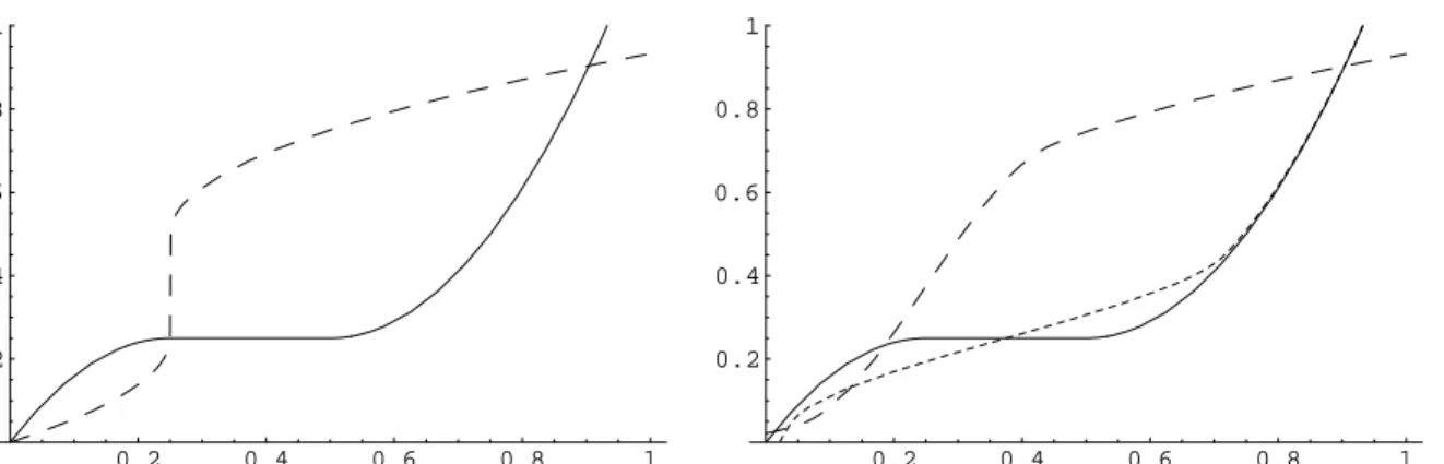
The following figures show the monotone modifications hI and hSI for a monotone (Figure 1) and a not everywhere monotone function h (Figure 2).

We will also give asymptotic results for discrete versions, ˆgI,d = Φ( ˜Φ(ˆg)I[ˆg(0),ˆg(1)])I[0,1] and

ˆ

gSI,d= Φ( ˜Ψ(ˆg)I[ˆg(0),gˆ(1)])I[0,1] where the integrals in the definitions of ˆgI and ˆgIS are

approx-imated by Riemann sums, i. e. ˜ Φ(g)(y) = 1 N N X i=1 I{ˆg( i N)≤y} ˜ Ψ(g)(y) = 1 N N X i=1 Ky−gˆ( i N) a .

For the estimator ˆgSI,d of a strictly increasing regression function Dette et al. (2005a) showed asymptotic normality under some regularity assumptions. One could also consider estimators

˜

Φ( ˜Φ(ˆg)I[ˆg(0),ˆg(1)])I[0,1]and ˜Φ( ˜Ψ(ˆg)I[ˆg(0),gˆ(1)])I[0,1]but for the second “inversion” a discretization

is not expedient as ˜Φ(ˆg) and ˜Ψ(ˆg) are already monotone and for a monotone function h we have just Φ(h) = inf{u|h(u)>·}.

0.2 0.4 0.6 0.8 1 0.2 0.4 0.6 0.8 1 0.2 0.4 0.6 0.8 1 0.2 0.4 0.6 0.8 1

Figure 1: The two graphics show isotone modifications of the nondecreasing functionh(x) = 0.25−4(x−0.25)2_{I{0 ≤x ≤0.25}+ 4(x−0.5)}2_{I{0.5≤ x≤ 1} (solid line). hI in the left}

panel is identical to h, the dotted line in the right panel is hSI for the Epanechnikov–kernel

k(x) = 0.75(1−x2_{)I{−1≤ x≤1} and bandwidth a = 0.2. The dashed curves are Φ(h) in}

the left panel and Ψ(h) in the right panel.

0.2 0.4 0.6 0.8 1 0.2 0.4 0.6 0.8 1 0.2 0.4 0.6 0.8 1 0.2 0.4 0.6 0.8 1

Figure 2: The two graphics show monotone modifications of the not monotone function

h(x) = 5x3 _{+ 4x − 8x}2 _{(solid line). The dotted lines are hI in the left panel and hSI}

in the right panel. For the calculation of hSI we used the Epanechnikov–kernel k(x) = 0.75(1−x2_{)I{−1≤x≤1} and bandwidth a= 0.2. The dashed curves are Φ(h) in the left}

3

Main results and applications

In this section we give conditions under which the increasing versions of function estimators share the same rate of uniform convergence as the original estimator. Let in the following

||h||∞= supz∈[0,1]|h(z)| denote the supremum norm of a function h: [0,1]→R.

Theorem 3.1 (a) Let g : [0,1] → R be an increasing function and gˆ : [0,1] → R an estimator for g. Then there exists a constant c such that for the isotone modification ˆgI of

ˆ

g it holds that

||gˆI−g||∞ ≤ c||gˆ−g||∞.

(b) Let g : [0,1] → R be a strictly increasing twice differentiable function with bounded second derivative such that the first derivative is bounded away from zero. Let ˆg : [0,1]→R

be an estimator for g. Let k denote a symmetric density function with compact support and two bounded derivatives. Let an=o(1)denote a sequence of positive bandwidths. Then there exists a constant csuch that for the strictly increasing modification ˆgSI of gˆit holds that

||gˆSI−g||∞ ≤ c ||ˆg−g||∞+ 1 an||gˆ−g|| 2 ∞+ 1 a3 n ||gˆ−g||3 ∞+a2n .

The constant cin Theorem 3.1 obtained in the proof is not claimed to be the best possible. In special cases (for example estimating a regression function by kernel methods) it might be possible to obtain sharper bounds, but our results are valid very general and the given proof is uncomplicated. In the situation of Theorem 3.1 (a) we obtain uniform consistency of the estimator ˆgI whenever ||ˆg−g||∞ = o(1) is known. Also, when rates of convergence

are known for the original estimator, i. e. ||ˆg−g||∞=O(cn) forn → ∞a.s. (in probability),

then the same holds for ˆgI, i. e.

||gIˆ −g||∞=O(cn) for n → ∞a.s. (in probability).

The estimator ˆgI based on the indicator method works better to estimate constant functions resp. nondecreasing functions with flat parts. Moreover, there is no need for choosing a bandwidth an when using this estimator.

In contrast, in the situation of Theorem 3.1 (b) uniform consistency of the estimator ˆgSI can

only be obtained from rates of the uniform convergence of ˆg and by choosing the bandwidth

an accordingly. When it is known that ||gˆ−g||∞ =O(cn) for n → ∞ a.s. (in probability),

then it holds that

||ˆgSI −g||∞=O cn+ c 2 n an + c3 n a3 n

+a2_n for n→ ∞ a.s. (in probability).

When a sequence of bandwidths an is chosen that satisfies cn = O(an5/3) and an = O(c1n/2)

we obtain the same rate O(cn) for the uniform convergence of the strictly increasing version. For the discrete versions we have the following asymptotic results.

Theorem 3.2 (a)Let g : [0,1]→Rbe a strictly increasing differentiable function such that the first derivative is bounded away from zero and let gˆ: [0,1] → R be an estimator for g. Then there exists a constant c such that for the isotone modification gˆI,d of gˆit holds that

||ˆgI,d−g||∞ ≤ c ||gˆ−g||∞+ 1 N .

(b) Let g : [0,1] → R be an strictly increasing twice differentiable function with bounded second derivative such that the first derivative is bounded away from zero. Let ˆg : [0,1]→R

an estimator for g. Let k denote a symmetric density function with compact support and two bounded derivatives. Let an=o(1)denote a sequence of positive bandwidths. Then there exists a constant csuch that for the strictly increasing modification ˆgSI,d of gˆit holds that

||gSI,dˆ −g||∞ ≤ c ||ˆg−g||∞(1 + 1 N an) + 1 an||gˆ−g|| 2 ∞(1 + 1 N a2 n ) + 1 a3 n ||gˆ−g||3_∞ + 1 N + 1 N2_an + 1 N3_a3 n +a2_n.

There are plenty of applications and we only mention a few. Whenever we have knowledge about uniform consistency of a function estimate and a monotone uniformly consistent esti-mator is desired it is sensible to use one of the above methods. For example, uniform almost sure consistency of kernel density estimators was shown by Silverman (1978), Devroye and Wagner (1978) and Stute (1982), among others. For kernel regression estimators correspond-ing results can be found in Mack and Silverman (1982), see also Einmahl and Mason (2000). Rates of uniform almost sure convergence for variance function estimators in nonparametric regression models are a by-product of Akritas and Van Keilegom (2001). Further, there is a vast literature about uniform consistency of wavelet estimators for densities and re-gression functions based on iid or time series or censored data, respectively, see, e. g., Masry (1997), Massiani (2003), Zhang, Sha and Cheng (1999) or Xue (2002). Corresponding results about orthogonal series estimators can be found in publications by Chen (1981), Gy¨orfi and Walk (1996), Newey (1997) and de Jong (2002). Moreover, strong uniform consistency of

k-nearest neighbor estimators for regression and density functions based on iid or dependent data is considered by Devroye and Wagner (1977), Mack (1983), and Qin and Cheng (1994). Uniform consistency for different estimators of hazard rates is shown by Zhang (1996) and Collomb, Hassani, Sarda and Vieu (1985). For each of the proposed estimators our method yields a monotone version that shares the same rate of uniform convergence.

For example, let m denote the isotone regression function in a nonparametric regression model

Yi = m(Xi) +εi, i= 1, . . . , n

with independent observations and univariate covariates Xi ∈ [0,1]. Let ˆm denote the common kernel regression estimator (Nadaraya, 1964; Watson, 1964),

ˆ m(x) = Pn i=1κ( x−Xi hn )Yi Pn i=1κ( x−Xi hn ) ,

where κ denotes a kernel function and hn a sequence of positive bandwidths converging to zero. Under common regularity assumptions (see Mack and Silverman, 1982) it holds that

||mˆ −m||∞=O(cn) for n→ ∞ a.s., where cn=

s

logh−1

n nhn .

We obtain an isotone modification of the kernel estimator ˆm, namely ˆmI. This estimator

fulfills ||mIˆ −m||∞=O(cn) forn → ∞ a.s. For the smooth version ˆmSI we obtain||mSIˆ −

m||∞ = O(cn) for n → ∞ a.s. when a sequence of bandwidths an is chosen that fulfills nhna4

n/logh−n1 =O(1) and logh−n1/(nhna

10/3

n ) =O(1). For the common choicehn=Cn−1/5,

for instance, an=hn is a possible choice. Note that Birke and Dette (2005) show a rate for uniform convergence of ˆm−_SI1 as a by-product.

Masry (1997) considers d–dimensional wavelet density estimators ˆf on compact sets D for strongly mixing stationary processes and densities f in certain Besov spaces Bspq. For sim-plicity we assume D = [0,1] and consider the one-dimensional case d = 1. For example, under certain assumptions in Corollary 1, Masry (1997) obtains the uniform rate of conver-gence ||fˆ−f||∞ = O logn n s 1+2s for n → ∞a.s.

forf ∈Bs∞∞. The wavelet estimator ˆf can be modified to obtain increasing (or, analogously,

decreasing) estimators ˆfI and ˆfSI such that

||fIˆ −f||∞ = O logn n s 1+2s and ||fSIˆ −f||∞ = O logn n s 1+2s for n → ∞ a.s. where for ˆfSIa bandwidthanis used such thatna4+2n /s/logn=O(1) and logn/(na2n/3+5/(3s)) = O(1). For example, an=Cn−1/5 is a possible choice for s= 2.

Finally, we consider how the assumption of the compact support of the target function can be weakened. For instance, often densities are assumed to be increasing on (−∞,0] (respectively decreasing on [0,∞)) and also hazard rates are often defined on [0,∞). We will describe in the following how the proposed methods are applicable when an increasing functionh: (−∞,0]→ Rhas to be estimated. Assume there is an estimator ˆh: (−∞,0]→R available such that

sup

z∈(−∞,0]

|ˆh(z)−h(z)|=O(cn).

Because log : (0,1] → (−∞,0] is continuous we have for g = h ◦log, ˆg = ˆh ◦log that

||ˆg−g||∞ = O(cn) and from the results of Sections 2 and 3 we obtain a monotone version

of ˆg, i. e. ˆgI, such that ||ˆgI −g||∞ = O(cn). A monotone estimator for h is defined by

ˆ

hI = ˆgI◦exp : (−∞,0]→Rand it holds that sup

z∈(−∞,0]

4

Proofs

4.1

Proof of Theorem 3.1 (a).

For increasing g we have g =gI and, hence,

||ˆgI−g||∞ = sup z∈[0,1] Z ˆg(1) ˆ g(0) InR1 0 I{gˆ(t)≤x}dt ≤z o dx+ ˆg(0) − Z g(1) g(0) InR1 0 I{g(t)≤x}dt≤z o dx−g(0) ≤ 2|gˆ(0)−g(0)|+|ˆg(1)−g(1)|+rn where rn = sup z∈[0,1] Z g(1) g(0) InR1 0 I{gˆ(t)≤x}dt≤z o −InR1 0 I{g(t)≤x}dt ≤z o dx ≤ sup z∈[0,1] Z g(1) g(0) InR1 0 I{gˆ(t)≤x}dt ≤z and R1 0 I{g(t)≤x}dt > z o dx + sup z∈[0,1] Z g(1) g(0) InR1 0 I{gˆ(t)≤x}dt > z and R1 0 I{g(t)≤x}dt≤z o dx.

Both summands are bounded in the very same way and we therefore restrict to the first one in the following, i. e. sup z∈[0,1] Z g(1) g(0) InR1 0 I{g(t)≤x−(ˆg(t)−g(t))}dt≤z < R1 0 I{g(t)≤x}dt o dx ≤ sup z∈[0,1] Z g(1) g(0) InR1 0 I{g(t)≤x− ||gˆ−g||∞}dt≤z < R1 0 I{g(t)≤x}dt o dx = sup z∈[0,1] Z g(1) g(0) Ing−1(x− ||gˆ−g||∞)≤z < g−1(x) o dx ≤ sup z∈[0,1] Z g(1) g(0) Ing(z)≤x≤g(z) +||ˆg−g||∞ o dx = sup z∈[0,1] Ing(z) +||ˆg−g||∞≤g(1) o ||ˆg−g||∞+I n g(z) +||ˆg−g||∞> g(1) o (g(1)−g(z)) ≤ ||gˆ−g||∞. Altogether we obtain ||ˆgI−g||∞ ≤ 2|gˆ(0)−g(0)|+|ˆg(1)−g(1)|+ 2||ˆg−g||∞ ≤ 5||ˆg−g||∞. 2

4.2

Proof of Theorem 3.1 (b).

For the proof of Theorem 3.1 (b) we first show that the following Proposition is valid.

Proposition 4.1 Let g : [0,1] → R be a strictly increasing twice differentiable function with bounded second derivative such that the first derivative is bounded away from zero. Let ˆg : [0,1] → _R be an estimator for g. Let k denote a symmetric density function with compact support and two bounded derivatives and let an =o(1) denote a sequence of positive bandwidths. Then there exists a constant C such that

sup y∈(g(0),g(1)) |Ψ(ˆg)(y)−g−1(y)| ≤ C||ˆg−g||∞+ 1 an||ˆg−g|| 2 ∞+ 1 a3 n ||gˆ−g||3_∞+a2_n Proof of Proposition 4.1. During the proof we assume the support of k to be [−1,1]. Note that then K(z) = 0 forz ≤ −1 andK(z) = 1 forz ≥1. For every fixedy∈(g(0), g(1)) we have |Ψ(ˆg)(y)−g−1(y)| ≤ Z 1 0 h Ky−gˆ(x) an −Ky−g(x) an i dx (4.1) + Z 1 0 Ky−g(x) an dx−g−1(y) .

The first term on the right hand side of (4.1) is estimated by a Taylor expansion,

Z 1 0 h Ky−gˆ(x) an −Ky−g(x) an i dx ≤ Z 1 0 1 ank y−g(x) an (ˆg(x)−g(x))dx + Z 1 0 1 a2 n k0y−g(x) an (ˆg(x)−g(x))2dx + sup u∈IR |k00(u)| 1 a3 n ||gˆ−g||3_∞ ≤ C1||ˆg−g||∞+C2 1 an||ˆg−g|| 2 ∞+C3 1 a3 n ||ˆg−g||3_∞

for some constants C1, C2, C3, where the last line follows by a replacement of variables,

z = (y−g(x))/an, in the integrals. By a change of the variable and integration by parts we obtain that the second term on the right hand side of (4.1) is bounded by

Z g−1(y−an) 0 Ky−g(x) an dx+ Z g−1(y+an) g−1_(y−a n) Ky−g(x) an dx−g−1(y) ≤ g −1_(y−an)− Z 1 −1 K(z) ∂ ∂zg −1_{(y−anz)dz−g}−1_(y) = g −1_(y−a n)−K(z)g−1(y−anz) z=1 z=−1+ Z 1 −1 k(z)g−1_(y−a nz)dz−g−1(y) ≤ a2_nsup t |(g−1)00(t)| Z k(z)z2dz ≤C4a2n

Proof of Theorem 3.1 (b). Denote Dn=C(||ˆg−g||∞+_a1n||gˆ−g|| 2 ∞+a13 n||gˆ−g|| 3 ∞+a2n)

such that supy∈(g(0),g(1))|Ψ(ˆg)(y)− g−1(y)| ≤ Dn from Proposition 4.1. Then from g =

Φ(g−1_I [g(0),g(1)])I[0,1] it follows that ||gSIˆ −g||∞ = sup z∈[0,1] Z ˆg(1) ˆ g(0) InΨ(ˆg)(x)≤zodx+ ˆg(0)− Z g(1) g(0) Ing−1(x)≤zodx−g(0) ≤ 2|gˆ(0)−g(0)|+|ˆg(1)−g(1)|+rn where rn ≤ sup z∈[0,1] Z g(1) g(0) InΨ(ˆg)(x)≤z < g−1(x)odx+ sup z∈[0,1] Z g(1) g(0) Ing−1(x)≤z <Ψ(ˆg)(x)odx.

Both summands are estimated in the very same way and by Proposition 4.1 the first one is bounded by sup z∈[0,1] Z g(1) g(0) Ing−1(x)−Dn ≤z < g−1(x)odx ≤ sup z∈[0,1] |g(z+Dn)−g(z)| ≤ ||g0||∞Dn.

The assertion follows collecting all bounds together. 2

4.3

Proof of Theorem 3.2 (a).

For the proof of Theorem 3.2 (a) we first show that the following Proposition is valid.

Proposition 4.2 Let g : [0,1]→R be a strictly increasing differentiable function such that the first derivative is bounded away from zero, and gˆ: [0,1]→ R an estimator for g. Then there exists a constant C such that

sup y∈(g(0),g(1)) |Φ(ˆ˜ g)(y)−g−1(y)| ≤ C||gˆ−g||∞+ 1 N . Proof of Proposition 4.2. We consider the following decomposition,

˜ Φ(g)(y)−g−1(y) = 1 N N X i=1 h I{gˆ( i N)≤y} −I{g( i N)≤y} i (4.2) + N X i=1 Z Ni i−1 N h I{g( i N)≤y} −I{g(x)≤y}dx i + Z 1 0 I{g(x)≤y}dx−g−1(y).

Because g is increasing, the last line vanishes. The absolute value of the second term on the right hand side of (4.2) can be bounded, for all y∈(g(0), g(1)), by

N X i=1 Z Ni i−1 N I{g(x)≤y < g( i N)}dx ≤ N X i=1 Z Ni i−1 N I{g(i−1 N )≤y≤g( i N)}dx ≤ N X i=1 1 NI{g −1_(y)≤ i N ≤g −1_{(y) +} 1 N}dx ≤ 2 N.

A bound for the absolute value of the first term on the right hand side of (4.2) is given by 1 N N X i=1 I{gˆ( i N)≤y≤g( i N)}+ 1 N N X i=1 I{g( i N)≤y ≤gˆ( i N)}

and we only consider the second term in the following. It is bounded by 1 N N X i=1 I{g( i N)≤y≤g( i N) +||ˆg−g||∞} ≤ 1 N N X i=1 I{g−1(y− ||gˆ−g||∞)≤ i N ≤g −1_(y)} ≤ 2g−1(y)−g−1(y− ||gˆ−g||∞) ≤ 2||1 g0||∞||gˆ−g||∞

for all y such thaty− ||ˆg−g||∞≥g(0). Otherwise we estimate

sup y∈[g(0),g(0)+||gˆ−g||∞] 1 N N X i=1 I{g( i N)≤y≤g( i N) +||gˆ−g||∞} ≤ 1 N]{i|g( i N)≤g(0) +||gˆ−g||∞} ≤ 2g−1_{(g(0) +||ˆg−g||} ∞) ≤ 2|| 1 g0||∞||ˆg−g||∞

and the assertion of the Proposition follows. 2

Proof of Theorem 3.2 (a). Theorem 3.2 (a) follows from Proposition 4.2 in the same way

as Theorem 3.1 (b) is deduced from Proposition 4.1. 2

4.4

Proof of Theorem 3.2 (b).

For the proof of Theorem 3.2 (b) we first show that the following Proposition is valid.

Proposition 4.3 Let g : [0,1] → R be a strictly increasing twice differentiable function with bounded second derivative such that the first derivative is bounded away from zero. Let ˆg : [0,1] → R be an estimator for g. Let k denote a symmetric density function with compact support and two bounded derivatives and let an =o(1) denote a sequence of positive bandwidths. Then there exists a constant C such that

sup y∈(g(0),g(1)) |Ψ(ˆ˜ g)(y)−g−1(y)| ≤ C||ˆg−g||∞(1 + 1 N an ) + 1 an ||gˆ−g||2_∞(1 + 1 N a2 n ) + 1 a3 n ||ˆg−g||3_∞+ 1 N + 1 N2_an + 1 N3_a3 n +a2_n Proof of Proposition 4.3. We have

|Ψ(ˆ˜ g)(y)−Ψ(ˆg)(y)| = 1 N N X i=1 h Ky−ˆg( i N) an −Ky−g( i N) an i (4.3) + N X i=1 Z Ni i−1 N h Ky−g( i N) an −Ky−g(x) an i dx

and by a Taylor expansion the first term on the right hand side of (4.3) is bounded by 1 N N X i=1 1 ank y−g(i N) an (g( i N)−gˆ( i N)) + 1 N N X i=1 1 a2 n k0y−g( i N) an (g( i N)−gˆ( i N)) 2 + sup u∈IR |k00(u)| 1 a3 n ||ˆg−g||3_∞ ≤ ||gˆ−g||∞ Z 1 ank y−g(x) an dx+ 1 an||gˆ−g|| 2 ∞ Z 1 an k 0y−g(x) an dx +||ˆg−g||∞ N X i=1 Z i/N (i−1)/N 1 an k y−g(i N) an −ky−g(x) an dx + 1 a2 n ||gˆ−g||2_∞ N X i=1 Z i/N (i−1)/N k 0y−g( i N) an −k0y−g(x) an dx + sup u∈IR |k00(u)| 1 a3 n ||ˆg−g||3_∞ ≤ C1 ||ˆg−g||∞(1 + 1 N an + 1 N2_a3 n ) + 1 an||ˆg−g|| 2 ∞(1 + 1 N a2 n ) + 1 a3 n ||ˆg−g||3_∞

for some constant C1, where the last inequality follows by similar calculations as in the

argumentation for the second term on the right hand side of (4.3). This one is bounded by

N X i=1 Z Ni i−1 N 1 ank y−g(x) an (g( i N)−g(x))dx + N X i=1 Z Ni i−1 N 1 a2 n k0y−g(x) an (g( i N)−g(x)) 2_dx + 1 a3 n sup u∈IR |k00(u)| N X i=1 Z Ni i−1 N |g( i N)−g(x)| 3_dx ≤ ||g0||∞ 1 N Z 1 0 1 ank y−g(x) an dx+ (||g0||∞ 1 N) 2Z 1 0 1 a2 n k 0y−g(x) an dx + sup u∈IR |k00(u)|(||g0||∞ 1 anN) 3 ≤ C2 1 N + 1 N2_an + 1 N3_a3 n

for some constant C2 uniformly with respect toy, where the last line follows from a change

of variable z = (y−g(x))/an in the integrals and because g−1 _{is bounded. The assertion}

now follows by Proposition 4.1. 2

Proof of Theorem 3.2 (b). Theorem 3.2 (b) follows from Proposition 4.3 in the same

Acknowledgements. This work was done while the author visited the Australian National University in Canberra and she would like to thank the members of the Mathematical Science Institute, in particular Peter Hall, for their hospitality.

5

References

M. Akritas and I. Van Keilegom (2001). Nonparametric estimation of the residual dis-tribution. Scand. J. Statist. 28, 549–567.

R. E. Barlow, D. J. Bartholomew, J. M. Bremmer and H. D. Brunk (1972). Statis-tical Inference under order restrictions. Wiley, New York.

M. Birke and H. Dette (2005). A note on estimating a monotone regression by combin-ing kernel and density estimates. preprint, http://www.rub.de/mathematik3/preprint.htm

H. D. Brunk (1958). On the estimation of parameters restricted by inequalities. Annals of Mathematical Statistics 29, 437–454.

T. W. Chen (1981). On the strong consistency of density estimation by orthogonal series methods. Tamkang J. Math. 12, 265–268.

M-Y. Cheng, T. Gasser and P. Hall (1999). Nonparametric density estimation under unimodality and monotonicity constraints. Journal of Computational and Graphical Statistics 8, 1–21.

G. Collomb, S. Hassani, P. Sarda, P. Vieu (1985). Convergence uniforme d’estimateurs de la fonction de hasard pour des observations d´ependantes: m´ethodes du noyau et des

k-points les plus proches. (French) [Strong uniform consistency of kernel andk-nearest neighbor estimates of the hazard rate from dependent observations]. C. R. Acad. Sci. Paris S´er. I Math. 301, 653–656.

S. Datta (1995). A minimax optimal estimator for continuous monotone densities. Journal of Statistical Planning and Inference 46, 183–193.

R. M. de Jong (2002). A note on: “Convergence rates and asymptotic normality for series estimators” [J. Econometrics 79 (1997), no. 1, 147–168] by W. K. Newey: uniform convergence rates. J. Econometrics 111, 1–9.

H. Dette, N. Neumeyer and K. Pilz (2005a). A simple nonparametric estimator of a strictly increasing regression function. forthcoming in Bernoulli.

http://www.rub.de/mathematik3/preprint.htm

H. Dette, N. Neumeyer and K. Pilz (2005b). A note on nonparametric estimation of the effective dose in quantal bioassay. forthcoming in Journal of the American Statis-tical Association. http://www.rub.de/mathematik3/preprint.htm

H. Dette, K. Pilz (2004). On the estimation of a monotone conditional variance in non-parametric regression. technical report Ruhr-Universit¨at Bochum.

http://www.ruhr-uni-bochum.de/mathematik3/preprint.htm

L. P. Devroye, T. J. Wagner (1977). The strong uniform consistency of nearest neighbor density estimates. Ann. Statist. 5, 536–540.

L. P. Devroye, T. J. Wagner (1978). The strong uniform consistency of kernel density estimates. Multivariate analysis, V (Proc. Fifth Internat. Sympos., Univ. Pittsburgh, Pittsburgh, Pa., 1978), pp. 59–77, North-Holland, Amsterdam-New York, 1980.

U. Einmahl, D. M. Mason (2000). An empirical process approach to the uniform consis-tency of kernel-type function estimators. J. Theoretical Probab. 13, 1–37.

I. Gijbels (2003). Monotone regression. Discussion paper 0334, Institute de Statistique, Universit´e Catholique de Louvain. http://www.stat.ucl.ac.be/ISpub/ISdp.html

U. Grenander (1956). On the theory of mortality measurement II. Skand. Aktuarietidskr. 39, 125–153.

P. Groeneboom (1985) Estimating a monotone density. Proceedings of the Berkeley conference in honor of Jerzy Neyman and Jack Kiefer, Vol. II (Berkeley, Calif., 1983), 539–555, Wadsworth Statistics/Probability Series.

P. Groeneboom and H. P. Lopuha¨a (1993). Isotonic estimators of monotone densities and distribution functions: basic facts. Statistica Neerlandica 47, 175–183.

L. Gy¨orfi, H. Walk (1996). On the strong universal consistency of a series type regression estimate. Math. Methods Statist. 5, 332–342.

P. Hall and L-S. Huang (2001). Nonparametric kernel regression subject to monotonicity constraints. Annals of Statistics 29, 624–647.

P. Hall, L-S. Huang, J. A. Gifford and I. Gijbels (2001). Nonparametric estimation of hazard rate under the constraint of monotonicity. Journal of Computational and Graphical Statistics 10, 592–614.

J. Huang and J. A. Wellner (1995). Estimation of a monotone density or monotone haz-ard under random censoring. Scandinavian Journal of Statistics 22, 3–33.

Y. Huang and C.–H. Zhang (1994). Estimating a monotone density from censored ob-servations. Annals of Statistics 22, 1256–1274.

Y. P. Mack (1983). Rate of strong uniform convergence of k-NN density estimates. J. Statist. Plann. Inference 8, 185–192.

Y. P. Mack, B. W. Silverman (1982). Weak and strong uniform consistency of kernel regression estimates. Z. Wahrsch. Verw. Gebiete 61, 405–415.

E. Mammen (1991). Estimating a smooth monotone regression function. Annals of Statis-tics 19, 724–740.

A. Massiani (2003). Vitesse de convergence uniforme presque sˆure de l’estimateur lin´eaire par m´ethode d’ondelettes. (French) [Rate of almost sure uniform convergence of the linear wavelet density estimator]. C. R. Math. Acad. Sci. Paris 337, 67–70.

E. Masry (1997). Multivariate probability density estimation by wavelet methods: strong consistency and rates for stationary time series. Stoch. Process. Appl. 67, 177–193.

H. Mukerjee (1988). Monotone nonparametric regression. Ann. Statist. 16, 741–750.

H. Mukerjee and J-L. Wang (1993). Nonparametric maximum likelihood estimation of an increasing hazard rate for uncertain cause-of-death data. Scandinavian Journal of Statistics 20, 17–33.

´

E. A. Nadaraya (1964). On non–parametric estimates of density functions and regression curves. J. Probab. Appl. 10, 186–190.

W. Newey (1997). Convergence rates and asymptotic normality for series estimators. J. Econometrics 79, 147–168.

W. Polonik (1995). Density estimation under qualitative assumptions in higher dimen-sions. J. Multivariate Anal. 55, 61–81.

W. Polonik (1998). The silhouette, concentration functions and ML-density estimation under order restrictions. Ann. Statist. 26, 1857–1877.

G. S. Qin, P. Cheng (1994). Strong uniform consistency of k-nearest neighbor regression function estimators. Sci. China Ser. A 37, 1032–1040.

J. O. Ramsay (1988). Monotone regression splines in action (with discussion). Statistical Science, 3, 425–441.

J. V. Ryff (1965). Orbits of L1_{-functions under doubly stochastic transformations. Trans.}

Americ. Math. Soc. 117, 92-100.

J. V. Ryff (1970). Measure preserving transformations and rearrangements. J. Math. Anal. Appl. 31, 449-458.

B. W. Silverman (1978). Weak and strong uniform consistency of the kernel estimate of a density and its derivatives. Ann. Statist. 6, 177–184.

R. T. Smythe (1980). Maxima of partial sums and a monotone regression estimator. Ann. Probab. 8, 630–635.

W. Stute (1982). A law of the logarithm for kernel density estimators. Ann. Probab. 10, 414–422.

A. B. Tsybakov (1997). On nonparametric estimation of density level sets. Ann. Statist. 25, 948–969.

A. W. van der Vaart and M. J. van der Laan (2003). Smooth estimation of a mono-tone density. Statistics 37, 189–203.

G. S. Watson (1964). Smooth Regression Analysis. Sankhya A 26, 359–372.

F. T. Wright (1979) A strong law for variables indexed by a partially ordered set with ap-plications to isotone regression. Ann. Probab. 7, 109–127.

L. G. Xue (2002). Strong uniform convergence rates of wavelet estimates of regression function under complete and censored data. Acta Math. Appl. Sin. 25, 430–438.

B. Zhang (1996). A note on strong uniform consistency of kernel estimators of hazard functions under random censorship. Lifetime data: models in reliability and survival analysis. (Cambridge, MA, 1994), 395–399, Kluwer Acad. Publ., Dordrecht, 1996.

S. L. Zhang, Q. Y. Sha, M. Y. Cheng (1999). Uniform strong consistency of nonlinear wavelet estimates of regression functions. Chinese J. Appl. Probab. Statist. 15, 375–380.