A Hierarchical Latent Variable Model for Data Visualization

A Hierarchical Latent Variable Model

for Data Visualization

Christopher M. Bishop and Michael E. Tipping

Abstract—Visualization has proven to be a powerful and widely-applicable tool for the analysis and interpretation of multivariate data. Most visualization algorithms aim to find a projection from the data space down to a two-dimensional visualization space. However, for complex data sets living in a high-dimensional space, it is unlikely that a single two-dimensional projection can reveal all of the interesting structure. We therefore introduce a hierarchical visualization algorithm which allows the complete data set to be visualized at the top level, with clusters and subclusters of data points visualized at deeper levels. The algorithm is based on a hierarchical mixture of latent variable models, whose parameters are estimated using the expectation-maximization algorithm. We demonstrate the principle of the approach on a toy data set, and we then apply the algorithm to the visualization of a synthetic data set in 12 dimensions obtained from a simulation of multiphase flows in oil pipelines, and to data in 36 dimensions derived from satellite images. A Matlab software implementation of the algorithm is publicly available from the World Wide Web.

Index Terms—Latent variables, data visualization, EM algorithm, hierarchical mixture model, density estimation, principal component analysis, factor analysis, maximum likelihood, clustering, statistics.

—————————— ✦ ——————————

1 INTRODUCTION

ANY algorithms for data visualization have been pro-posed by both the neural computing and statistics communities, most of which are based on a projection of the data onto a two-dimensional visualization space. While such algorithms can usefully display the structure of simple data sets, they often prove inadequate in the face of data sets which are more complex. A single two-dimensional projection, even if it is nonlinear, may be insufficient to capture all of the interesting aspects of the data set. For ex-ample, the projection which best separates two clusters may not be the best for revealing internal structure within one of the clusters. This motivates the consideration of a hierarchical model involving multiple two-dimensional visualization spaces. The goal is that the top-level projec-tion should display the entire data set, perhaps revealing the presence of clusters, while lower-level projections dis-play internal structure within individual clusters, such as the presence of subclusters, which might not be apparent in the higher-level projections.

Once we allow the possibility of many complementary visualization projections, we can consider each projection model to be relatively simple, for example, based on a lin-ear projection, and compensate for the lack of flexibility of individual models by the overall flexibility of the complete hierarchy. The use of a hierarchy of relatively simple mod-els offers greater ease of interpretation as well as the bene-fits of analytical and computational simplification. This

philosophy for modeling complexity is similar in spirit to the “mixture of experts” approach for solving regression problems [1].

The algorithm discussed in this paper is based on a form of latent variable model which is closely related to both principal component analysis (PCA) and factor analysis. At the top level of the hierarchy we have a single visualization plot corresponding to one such model. By considering a probabilistic mixture of latent variable models we obtain a soft partitioning of the data set into “clusters,” corresponding to the second level of the hier-archy. Subsequent levels, obtained using nested mixture representations, provide successively refined models of the data set. The construction of the hierarchical tree proceeds top down, and can be driven interactively by the user. At each stage of the algorithm the relevant model parameters are determined using the expectation-maximization (EM) algorithm.

In the next section, we review the latent-variable model, and, in Section 3, we discuss the extension to mixtures of such models. This is further extended to hierarchical mix-tures in Section 4, and is then used to formulate an interac-tive visualization algorithm in Section 5. We illustrate the operation of the algorithm in Section 6 using a simple toy data set. Then we apply the algorithm to a problem in-volving the monitoring of multiphase flows along oil pipes in Section 7 and to the interpretation of satellite im-age data in Section 8. Finally, extensions to the algorithm, and the relationships to other approaches, are discussed in Section 9.

2 LATENT VARIABLES

We begin by introducing a simple form of linear latent vari-able model and discussing its application to data analysis. Here we give an overview of the key concepts, and leave 0162-8828/98/$10.00 © 1998 IEEE

————————————————

• C.M. Bishop is with Microsoft Research, St. George House, 1 Guildhall Street, Cambridge CB2 3NH, U.K. E-mail: [email protected].

• M.E. Tipping is with the Neural Computing Research Group, Aston Uni-versity, Birmingham B4 7ET, U.K. E-mail: [email protected]. Manuscript received 3 Apr. 1997; revised 23 Jan. 1998. Recommended for accep-tance by R.W. Picard.

For information on obtaining reprints of this article, please send e-mail to: [email protected], and reference IEEECS Log Number 106323.

M

the detailed mathematical discussion to Appendix A. The aim is to find a representation of a multidimensional data set in terms of two latent (or “hidden”) variables. Suppose the data space is d-dimensional with coordinates y1, º, yd

and that the data set consists of a set of d-dimensional vectors {tn} where n = 1, º, N. Now consider a

two-dimensional latent space x= (x1, x2) T

together with a lin-ear function which maps the latent space into the data space

y = Wx + m (1) where W is a d¥ 2 matrix and m is a d-dimensional vector. The mapping (1) defines a two-dimensional planar sur-face in the data space. If we introduce a prior probability distribution p(x) over the latent space given by a zero-mean Gaussian with a unit covariance matrix, then (1) defines a singular Gaussian distribution in data space with mean m and covariance matrix ·(y-m)(y -m)TÒ= WWT. Fi-nally, since we do not expect the data to be confined ex-actly to a two-dimensional sheet, we convolve this distri-bution with an isotropic Gaussian distridistri-bution p(t|x, s2) in data space, having a mean of zero and covariance s2I, where I is the unit matrix. Using the rules of probability, the final density model is obtained from the convolution of the noise model with the prior distribution over latent space in the form

p( ) =t

z

p( | ) ( ) t x px xd . (2) Since this represents the convolution of two Gaussians, the integral can be evaluated analytically, resulting in a distri-bution p(t) which corresponds to a d-dimensional Gaussian with mean mand covariance matrix WWT + s2I.

If we had considered a more general model in which the conditional distribution p(t|x) is given by a Gaussian with a general diagonal covariance matrix (having d independ-ent parameters), then we would obtain standard linear factor analysis [2], [3]. In fact, our model is more closely related to principal component analysis, as we now discuss. The log likelihood function for this model is given by L = Ân ln p(tn), and maximum likelihood can be used to fit the

model to the data and hence determine values for the pa-rameters m, W, and s2. The solution for mis just given by the sample mean. In the case of the factor analysis model, the determination of W and s2 corresponds to a nonlinear optimization which must be performed iteratively. For the isotropic noise covariance matrix, however, it was shown by Tipping and Bishop [4], [5] that there is an exact closed form solution as follows. If we introduce the sample co-variance matrix given by

S= t - t -=

Â

1 1 N n n n N m m

c

hc

h

T , (3) then the only nonzero stationary points of the likelihood occur for:

W = U (L-s2I)1/2R, (4)

where the two columns of the matrix U are eigenvectors of S, with corresponding eigenvalues in the diagonal ma-trix L, and R is an arbitrary 2 ¥ 2 orthogonal rotation ma-trix. Furthermore, it was shown that the stationary point corresponding to the global maximum of the likelihood occurs when the columns of U comprise the two principal eigenvectors of S (i.e., the eigenvectors corresponding to the two largest eigenvalues) and that all other combina-tions of eigenvectors represent saddle-points of the likeli-hood surface. It was also shown that the maximum-likelihood estimator of s2 is given by

s_ML2 l 3 1 2 = -=

Â

d j j d , (5) which has a clear interpretation as the variance “lost” in the projection, averaged over the lost dimensions.

Unlike conventional PCA, however, our model defines a probability density in data space, and this is important for the subsequent hierarchical development of the model. The choice of a radially symmetric rather than a more general diagonal covariance matrix for p(t|x) is motivated by the desire for greater ease of interpretability of the visualization results, since the projections of the data points onto the latent plane in data space correspond (for small values of s2) to an orthogonal projection as dis-cussed in Appendix A.

Although we have an explicit solution for the maximum-likelihood parameter values, it was shown by Tipping and Bishop [4], [5] that significant computational savings can sometimes be achieved by using the following EM (expec-tation-maximization) algorithm [6], [7], [8]. Using (2), we can write the log likelihood function in the form

L p _{n n} p d n N n n =

Â

z

= ln

d

t x

i c h

x x 1 , (6)

in which we can regard the quantities x_n as missing vari-ables. The posterior distribution of the xn, given the

ob-served tn and the model parameters, is obtained using

Bayes’ theorem and again consists of a Gaussian distribu-tion. The E-step then involves the use of “old” parameter values to evaluate the sufficient statistics of this distribu-tion in the form

·xnÒ=M

-1

WT(tn-m) (7)

x x_{n n}T =s2M-1+ x_n x_nT , (8) where M= WTW + s2I is a 2 ¥ 2 matrix, and · Ò denotes the expectation computed with respect to the posterior distri-bution of x. The M-step then maximizes the expectation of the complete-data log likelihood to give

~ W=

L

t - x x x

N

M

M

O

Q

P

P

L

N

M

M

O

Q

P

P

= =

-Â

n n

Â

n N n n n N m

c

h

T T 1 1 1 (9) ~ s2 = 1 2 2 1 Nd n n n n n n N t - + W W x x - x W t -=

Â

_{

m Tr

_e

~ ~T T

_j

T ~T

c

m

h

_}

(10)

in which ~ denotes “new” quantities. Note that the new value for W ~ obtained from (9) is used in the evaluation of s2 in (10). The model is trained by alternately evaluating the sufficient statistics of the latent-space posterior distri-bution using (7) and (8) for given s2 and W (the E-step), and re-evaluating s2 and W using (9) and (10) for given ·xnÒand x xn n

T

(the M-step). It can be shown that, at each stage of the EM algorithm, the likelihood is increased un-less it is already at a local maximum, as demonstrated in Appendix E.

For N data points in d dimensions, evaluation of the sample covariance matrix requires O(Nd2) operations, and so any approach to finding the principal eigenvectors based on an explicit evaluation of the covariance matrix must have at least this order of computational complexity. By contrast, the EM algorithm involves steps which are only

O(Nd). This saving of computational cost is a consequence of having a latent space whose dimensionality (which, for the purposes of our visualization algorithm, is fixed at two) does not scale with d.

If we substitute the expressions for the expectations given by the E-step equations (7) and (8) into the M-step equations we obtain the following re-estimation formulas

~ W = SW(s2I + M-1WTSW)-1 (11) ~ ~ s2 = 1 - -1 dTr T S SWM W

o

t

(12) which shows that all of the dependence on the data occurs through the sample covariance matrix S. Thus the EM algo-rithm can be expressed as alternate evaluations of (11) and (12). (Note that (12) involves a combination of “old” and “new” quantities.) This form of the EM algorithm has been introduced for illustrative purposes only, and would in-volve O(Nd2) computational cost due to the evaluation of the covariance matrix.

We have seen that each data point tninduces a Gaussian

posterior distribution p(xn|tn) in the latent space. For the

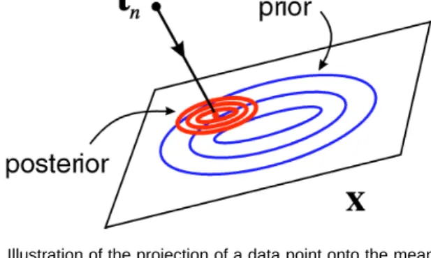
purposes of visualization, however, it is convenient to summarize each such distribution by its mean, given by ·xnÒ, as illustrated in Fig. 1. Note that these quantities are

obtained directly from the output of the E-step (7). Thus, a set of data points {tn} where n = 1, º, N is projected onto a

corresponding set of points {·x_nÒ} in the two-dimensional latent space.

3 MIXTURES OF LATENT VARIABLE MODELS

We can perform an automatic soft clustering of the data set, and at the same time obtain multiple visualization plots corresponding to the clusters, by modeling the data with a mixture of latent variable models of the kind de-scribed in Section 2. The corresponding density model takes the form

p _ip i i M t t

a f

=

c h

=

Â

p 1 0 (13)

where M0 is the number of components in the mixture, and

the parameters pi are the mixing coefficients, or prior

prob-abilities, corresponding to the mixture components p(t|i). Each component is an independent latent variable model with parameters mi, Wi, and si

2

. This mixture distribution will form the second level in our hierarchical model.

The EM algorithm can be extended to allow a mixture of the form (13) to be fitted to the data (see Appendix B for details). To derive the EM algorithm we note that, in addi-tion to the {xn}, the missing data now also includes labels

which specify which component is responsible for each data point. It is convenient to denote this missing data by a set of variables zni where zni = 1 if tn was generated by

model i (and zero otherwise). The prior expectations for these variables are given by the p_i and the corresponding posterior probabilities, or responsibilities, are evaluated in the extended E-step using Bayes’ theorem in the form

R P i p i p i ni n i n i i n = = Â_{¢ ¢} ¢ t t t

d i

c h

c

h

p p . (14) Although a standard EM algorithm can be derived by treating the {xn} and the zni jointly as missing data, a more

efficient algorithm can be obtained by considering a two-stage form of EM. At each complete cycle of the algorithm we commence with an “old” set of parameter values p_i, m_i,

Wi, and si

2

. We first use these parameters to evaluate the posterior probabilities Rni using (14). These posterior

prob-abilities are then used to obtain “new” values ~p_i and ~mi

using the following re-estimation formulas ~ p_{i ni} n N R = 1

Â

(15) ~ mi n ni n n ni R R = Â Â t . (16) The new values ~m_i are then used in evaluation of the suffi-cient statistics for the posterior distribution for xni

x_ni =M W t-_i1 _iT

c

_n -~m_i

h

(17)

x x_{ni ni}T =s_i2M_i-1+ x_ni x_niT (18) where M_i =W W_iT _i+s_i2I. Finally, these statistics are used to evaluate “new” values W~_i and ~s_i2 using

Fig. 1. Illustration of the projection of a data point onto the mean of the posterior distribution in latent space.

~ ~ W_{i ni} t_{n i} x_ni x x n ni ni ni n R R =

L

-N

M

M

O

Q

P

P

L

N

M

M

O

Q

P

P

Â

Â

-m

c

h

T T 1 (19) ~ ~ s_i n ni _n ni n i d R R 2 1 2 = t Â

R

S

|

T|

Â

-m - - +

U

_V

|

W|

Â

Â

2 R_ni R n ni i n i ni ni ni i i n xT W t~T

c

~m

h

Tr x xT W W~ ~T (20) which are derived in Appendix B.

As for the single latent variable model, we can substitute the expressions for ·xniÒand x xni ni

T

, givenby (17) and (18), respectively, into (19) and (20). We then see that the re-estimation formulae for W~_i and ~s_i2 take the form

~ W_i =S W_{i i}

e

s_i2I+M W S W_i-1 _iT _{i i}

j

-1 (21) ~ ~ s_{i i i i i i} d 2 ₌ 1 _- -1 Tr

e

S S W M WT

j

, (22) where all of the data dependence been expressed in terms of the quantities

S_i t t

i _n ni n i n i

N R

= 1

Â

c

-~_m

hc

-~_m

h

T, (23) and we have defined Ni = ÂnRni. The matrix Si can clearly

be interpreted as a responsibility weighted covariance ma-trix. Again, for reasons of computational efficiency, the form of EM algorithm given by (17) to (20) is to be pre-ferred if d is large.

4 HIERARCHICAL MIXTURE MODELS

We now extend the mixture representation of Section 3 to give a hierarchical mixture model. Our formulation will be quite general and can be applied to mixtures of any para-metric density model.

So far we have considered a two-level system consisting of a single latent variable model at the top level and a mixture of M0 such models at the second level. We can now

extend the hierarchy to a third level by associating a group

*i of latent variable models with each model i in the second

level. The corresponding probability density can be written in the form p _{i j i}p i j j i M i t t

a f

=

d

i

Π=

Â

Â

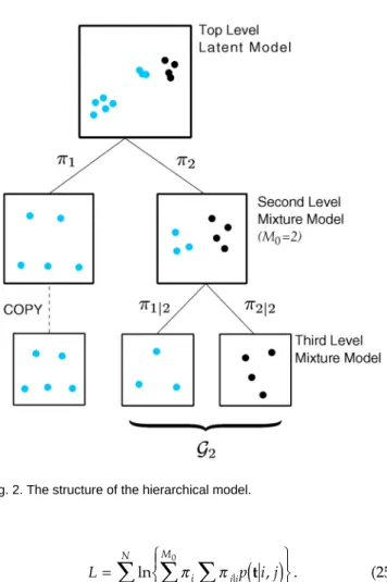
p p , * 1 0 , (24) where p(t|i, j)again represent independent latent variable models, andp_j|i correspond to sets of mixing coefficients, one for each i, which satisfy Âjpj|i = 1. Thus, each level of

the hierarchy corresponds to a generative model, with lower levels giving more refined and detailed representa-tions. This model is illustrated in Fig. 2.

Determination of the parameters of the models at the third level can again be viewed as a missing data problem in which the missing information corresponds to labels specifying which model generated each data point. When no information about the labels is provided the log likeli-hood for the model (24) would take the form

L _{i j i}p i j j i M n N i =

R

S

|

T|

U

V

|

W|

Π= =

Â

Â

Â

ln p p

d

t ,

i

* 1 1 0 . (25) If, however, we were given a set of indicator variables zni

specifying which model i at the second level generated each data point tnthen the log likelihood would become

L z_ni p i j i M i j i j n N i =

R

S

|

T|

U

V

|

W|

= Π=

Â

Â

Â

1 1 0 ln p p

d

t ,

i

* . (26) In fact, we only have partial, probabilistic, information in the form of the posterior responsibilities Rni for each model

i having generated the data points tn, obtained from the

second level of the hierarchy. Taking the expectation of (26), we then obtain the log likelihood for the third level of the hierarchy in the form

L R_ni p i j i M i j i j n N i =

R

S

|

T|

U

V

|

W|

= Π=

Â

Â

Â

1 1 0 ln p p

d

t ,

i

* , (27) in which the R_ni are constants. In the particular case in which the Rni are all 0 or 1, corresponding to complete

cer-tainty about which model in the second level is responsible for each data point, the log likelihood (27) reduces to the form (26).

Maximization of (27) can again be performed using the EM algorithm, as discussed in Appendix C. This has the same form as the EM algorithm for a simple mixture, discussed in Section 3, except that in the E-step, the poste-rior probability that model (i, j) generated data point tn is

given by

Rni,j = RniRnj|i, (28) in which R p i j p i j nj i j i n j j i n = Â_{¢ ¢} ¢ p p t t , ,

d

i

d

i

. (29)

Note that Rni are constants determined from the second

level of the hierarchy, and R_nj|i are functions of the “old” parameter values in the EM algorithm. The expression (29) automatically satisfies the relation

R_{ni j} R j ni i , Œ

Â

= * (30) so that the responsibility of each model at the second level for a given data point n is shared by a partition of unity between the corresponding group of offspring models at the third level.

The corresponding EM algorithm can be derived by a straightforward extension of the discussion given in Sec-tion 3 and Appendix B, and is outlined in Appendix C. This shows that the M-step equations for the mixing coefficients and the means are given by

~ , p_{j i} n ni j n ni R R = Â Â , (31) ~ , , , mi j n ni j n n ni j R R = Â Â t . (32) The posterior expectations for the missing variables z_ni,j are then given by

x_{ni j,} =M W-_{i j,}1 _{i j}T_,

e

t_n-~m_{i j,}

j

(33)

x_{ni j ni j,} xT_, =s2_{i j,}M_{i j}-_,1+ x_{ni j,} xT_{ni j,} (34) Finally, the Wi,j and si j,

2

are updated using the M-step equations ~ _~ , , , , , , , W_{i j ni j} t_{n i j} x_{ni j} x x n ni j ni j ni j n R R =

L

-N

M

M

O

Q

P

P

L

N

M

M

O

Q

P

P

Â

Â

-m

e

j

T T 1 (35) ~ ~ , , , , s_{i j} n ni j _n ni j n i j d R R 2 ₌ 1 2 Â

-R

S

|

T|

Â

t m - 2

Â

Rni j -n ni j i j n i j , , , , ~ ~ xT WT

e

t m

j

+

U

V

|

W|

Â

R_{ni j} n ni j ni j i j i j , , , , , ~ ~ Tr x xT W WT . (36) Again, we can substitute the E-step equations into the M-step equations to obtain a set of update formulas of the form ~ , , , , , , , , W_{i j} =S W_{i j i j}

e

s_{i j}2I+M W S W-_{i j}1 _{i j i j}T _{i j}

j

-1 (37) ~ ~ , , , , , , s_{i j i j i j i j i j i j} d 2 ₌ 1 _- -1 Tr

e

S S W M WT

j

(38) where all of the summations over n have been expressed in terms of the quantities

S_{i j} t t i j _n ni j n i j n i j N R , , , , , ~ ~ = 1

Â

e

-m

je

-m

j

T (39) in which we have defined N_i,j = Â_nR_ni,j. The S_i,j can again be interpreted as responsibility-weighted covariance matrices.

It is straightforward to extend this hierarchical modeling technique to any desired number of levels, for any para-metric family of component distributions.

5 THE VISUALIZATION ALGORITHM

So far, we have described the theory behind hierarchical mixtures of latent variable models, and have illustrated the overall form of the visualization hierarchy in Fig. 2. We now complete the description of our algorithm by consid-ering the construction of the hierarchy, and its application to data visualization.

Although the tree structure of the hierarchy can be pre-defined, a more interesting possibility, with greater practi-cal applicability, is to build the tree interactively. Our multi-level visualization algorithm begins by fitting a single la-tent variable model to the data set, in which the value of

m is given by the sample mean. For low values of the data space dimensionality d, we can find W and s2 directly by evaluating the covariance matrix and applying (4) and (5). However, for larger values of d, it may be computationally more efficient to apply the EM algorithm, and a scheme for initializing W and s2 is given in Appendix D. Once the EM algorithm has converged, the visualization plot is gener-ated by plotting each data point tn at the corresponding

posterior mean ·xnÒ in latent space.

On the basis of this plot, the user then decides on a suit-able number of models to fit at the next level down, and selects points x(i) on the plot corresponding, for example, to the centers of apparent clusters. The resulting points y(i)in data space, obtained from (1), are then used to initialize the means mi of the respective submodels. To initialize the

re-maining parameters of the mixture model, we first assign the data points to their nearest mean vector mi, and then

either compute the corresponding sample covariance ma-trices and apply a direct eigenvector decomposition, or use the initialization scheme of Appendix D followed by the EM algorithm.

Having determined the parameters of the mixture model at the second level we can then obtain the corre-sponding set of visualization plots, in which the posterior means ·xniÒ are again used to plot the data points. For

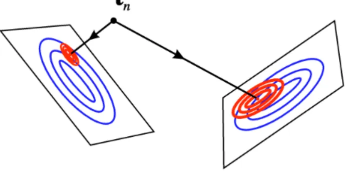
these, it is useful to plot all of the data points on every plot, but to modify the density of “ink” in proportion to the responsibility which each plot has for that particular data point. Thus, if one particular component takes most of the responsibility for a particular point, then that point will effectively be visible only on the corresponding plot. The projection of a data point onto the latent spaces for a mixture of two latent variable models is illustrated sche-matically in Fig. 3.

Fig. 3. Illustration of the projection of a data point onto the latent spaces of a mixture of two latent variable models.

The resulting visualization plots are then used to select further submodels, if desired, with the responsibility weighting of (28) being incorporated at this stage. If it is decided not to partition a particular model at some level, then it is easily seen from (30) that the result of training is equivalent to copying the model down unchanged to the next level. Equation (30) further ensures that the combina-tion of such copied models with those generated through further submodeling defines a consistent probability model, such as that represented by the lower three models in Fig. 2. The initialization of the model parameters is by direct analogy with the second-level scheme, with the co-variance matrices now also involving the responsibilities

Rni as weighting coefficients, as in (23). Again, each data

point is in principle plotted on every model at a given level, with a density of “ink” proportional to the corresponding posterior probability, given, for example, by (28) in the case of the third level of the hierarchy.

Deeper levels of the hierarchy involve greater numbers of parameters, and it is therefore important to avoid over-fitting and to ensure that the parameter values are well-determined by the data. If we consider principal compo-nent analysis, then we see that three (noncolinear) data points are sufficient to ensure that the covariance matrix has rank two and hence that the first two principal compo-nents are defined, irrespective of the dimensionality of the data set. In the case of our latent variable model, four data points are sufficient to determine both W and s2. From this, we see that we do not need excessive numbers of data points in each leaf of the tree, and that the dimensionality of the space is largely irrelevant.

Finally, it is often also useful to be able to visualize the spatial relationship between a group of models at one level and their parent at the previous level. This can be done by considering the orthogonal projection of the la-tent plane in data space onto the corresponding plane of the parent model, as illustrated in Fig. 4. For each model in the hierarchy (except those at the lowest level), we can plot the projections of the associated models from the level below.

In the next section, we illustrate the operation of this al-gorithm when applied to a simple toy data set, before pre-senting results from the study of more realistic data in Sec-tions 7 and 8.

6 ILLUSTRATION USING TOY DATA

We first consider a toy data set consisting of 450 data points generated from a mixture of three Gaussians in a three-dimensional space. Each Gaussian is relatively flat (has small variance) in one dimension, and all have the same covariance but differ in their means. Two of these pancake-like clusters are closely spaced, while the third is well sepa-rated from the first two. The structure of this data set has been chosen order to illustrate the interactive construction of the hierarchical model.

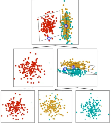
To visualize the data, we first generate a single top-level latent variable model, and plot the posterior mean of each data point in the latent space. This plot is shown at the top of Fig. 5, and clearly suggests the presence of two distinct clusters within the data. The user then selects two initial cluster centers within the plot, which initialize the sec-ond-level. This leads to a mixture of two latent variable models, the latent spaces of which are plotted at the sec-ond level in Fig. 5. Of these two plots, that on the right shows evidence of further structure, and so a submodel is generated, again based on a mixture of two latent variable models, which illustrates that there are indeed two fur-ther distinct clusters.

At this third step of the data exploration, the hierarchi-cal nature of the approach is evident as the latter two models only attempt to account for the data points which have already been modeled by their immediate ancestor. Indeed, a group of offspring models may be combined with the siblings of the parent and still define a consistent density model. This is illustrated in Fig. 5, in which one of the second level plots has been “copied down” (shown by the dotted line) and combined with the other third-level models. When offspring plots are generated from a par-ent, the extent of each offspring latent space (i.e., the axis limits shown on the plot) is indicated by a projected rec-tangle within the parent space, using the approach illus-trated in Fig. 4, and these rectangles are numbered se-quentially such that the leftmost submodel is “1.” In order to display the relative orientations of the latent planes, this number is plotted on the side of the rectangle which corresponds to the top of the corresponding offspring plot. The original three clusters have been individually colored, and it can be seen that the red, yellow, and blue data Fig. 4. Illustration of the projection of one of the latent planes onto its parent plane.

points have been almost perfectly separated in the third level.

7 OIL

FLOW

DATA

As an example of a more complex problem, we consider a data set arising from a noninvasive monitoring system used to determine the quantity of oil in a multiphase pipeline containing a mixture of oil, water, and gas [9]. The diagnostic data is collected from a set of three hori-zontal and three vertical beam-lines along which gamma rays at two different energies are passed. By measuring the degree of attenuation of the gammas, the fractional path length through oil and water (and, hence, gas) can readily be determined, giving 12 diagnostic measure-ments in total. In practice, the aim is to solve the inverse problem of determining the fraction of oil in the pipe. The complexity of the problem arises from the possibility of the multiphase mixture adopting one of a number of dif-ferent geometrical configurations. Our goal is to visualize the structure of the data in the original 12-dimensional space. A data set consisting of 1,000 points is obtained synthetically by simulating the physical processes in the pipe, including the presence of noise dominated by pho-ton statistics. Locally, the data is expected to have an in-trinsic dimensionality of two corresponding to the two degrees of freedom given by the fraction of oil and the

fraction of water (the fraction of gas being redundant). However, the presence of different flow configurations, as well as the geometrical interaction between phase boundaries and the beam paths, leads to numerous dis-tinct clusters. It would appear that a hierarchical ap-proach of the kind discussed here should be capable of discovering this structure. Results from fitting the oil flow data using a three-level hierarchical model are shown in Fig. 6.

In the case of the toy data discussed in Section 6, the optimal choice of clusters and subclusters is relatively unambiguous and a single application of the algorithm is sufficient to reveal all of the interesting structure within the data. For more complex data sets, it is appropriate to adopt an exploratory perspective and investigate alterna-tive hierarchies, through the selection of differing num-bers of clusters and their respective locations. The exam-ple shown in Fig. 6 has clearly been highly successful. Note how the apparently single cluster, number 2, in the top-level plot is revealed to be two quite distinct clusters at the second level, and how data points from the “homo-geneous” configuration have been isolated and can be seen to lie on a two-dimensional triangular structure in the third level.

Fig. 5. A summary of the final results from the toy data set. Each data point is plotted on every model at a given level, but with a density of ink which is proportional to the posterior probability of that model for the given data point.

8 SATELLITE IMAGE DATA

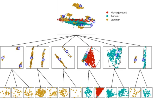
As a final example, we consider the visualization of a data set obtained from remote-sensing satellite images. Each data point represents a 3 ¥ 3 pixel region of a satellite land image, and, for each pixel, there are four measurements of intensity taken at different wavelengths (approximately red and green in the visible spectrum, and two in the near infrared). This gives a total of 36 variables for each data point. There is also a label indicating the type of land repre-sented by the central pixel. This data set has previously been the subject of a classification study within the STATLOG project [10].

We applied the hierarchical visualization algorithm to 600 data points, with 100 drawn at random of each of six classes in the 4,435-point data set. The result of fitting a three-level hierarchy is shown in Fig. 7. Note that the class labels are used only to color the data points and play no role in the maximum likelihood determination of the model parameters. Fig. 7 illustrates that the data can be approximately separated into classes, and the “gray soil” Æ “damp gray soil” Æ “very damp gray soil” continuum is clearly evident in component 3 at the second level. One particularly interesting additional feature is that there appear to be two distinct and separated clusters of “cot-ton crop” pixels, in mixtures 1 and 2 at the second level, which are not evident in the single top-level projection. Study of the original image [10] indeed indicates that there are two separate areas of “cotton crop.”

9 DISCUSSION

We have presented a novel approach to data visualization which is both statistically principled and which, as illus-trated by real examples, can be very effective at revealing structure within data. The hierarchical summaries of Figs. 5, 6, and 7 are relatively simple to interpret, yet still convey considerable structural information.

It is important to emphasize that in data visualization there is no objective measure of quality, and so it is difficult to quantify the merit of a particular data visualization tech-nique. This is one reason, no doubt, why there is a multi-tude of visualization algorithms and associated software available. While the effectiveness of many of these tech-niques is often highly data-dependent, we would expect the hierarchical visualization model to be a very useful tool for the visualization and exploratory analysis of data in many applications.

In relation to previous work, the concept of subsetting, or isolating, data points for further investigation can be traced back to Maltson and Dammann [11], and was further developed by Friedman and Tukey [12] for exploratory data analysis in conjunction with projection pursuit. Such subsetting operations are also possible in current dynamic visualization software, such as “XGobi” [13]. However, in these approaches there are two limitations. First, the parti-tioning of the data is performed in a hard fashion, while the mixture of latent variable models approach discussed in this paper permits a soft partitioning in which data points can effectively belong to more than one cluster at any given level. Second, the mechanism for the partitioning of the data is prone to suboptimality as the clusters must be fixed Fig. 6. Results of fitting the oil data. Colors denote different multiphase flow configurations corresponding to homogeneous (red), annular (blue), and laminar (yellow).

by the user based on a single two-dimensional projection. In the hierarchical approach advocated in this paper, the user selects only a “first guess” for the cluster centers in the mixture model. The EM algorithm is then utilized to de-termine the parameters which maximize the likelihood of the model, thus allowing both the centers and the widths of the clusters to adapt to the data in the full multidimen-sional data space. There is also some similarity between our method and earlier hierarchical methods in script recogni-tion [14] and morecogni-tion planning [15] which incorporate the Kohonen Self-Organizing Feature Map [16] and so offer the potential for visualization. As well as again performing a hard clustering, a key distinction in both of these ap-proaches is that different levels in the hierarchies operate on different subsets of input variables and their operation is thus quite different from the hierarchical algorithm de-scribed in this paper.

Our model is based on a hierarchical combination of linear latent variable models. A related latent variable technique called the generative topographic mapping (GTM) [17] uses a nonlinear transformation from latent space to data space and is again optimized using an EM algorithm. It is straightforward to incorporate GTM in place of the linear latent variable models in the current hierarchical framework.

As described, our model applies to continuous data variables. We can easily extend the model to handle dis-crete data as well as combinations of disdis-crete and con-tinuous variables. In case of a set of binary data vari-ables ykΠ{0, 1}, we can express the conditional distribution

of a binary variable, given x, using a binomial distribution

of the form p

c h

t x = ’_ks

e

w x_kT +m_k

j

tk 1-s

e

w xT_k +m_k

j

1-tk, wheres(a) = (1 + exp(-a))-1 is the logistic sigmoid function, and wk is thekth column of W. For data having a 1-of-D

coding scheme we can represent the distribution of data variables using a multinomial distribution of the form

p

c h

_{t x = ’}D_k m_kxk

=1 where mk are defined by a softmax, or

normalized exponential, transformation of the form

m_k k k j j j = + Â + exp exp w x w x T T m m

e

j

e

j

. (40)

If we have a data set consisting of a combination of con-tinuous, binary and categorical variables, we can formulate the appropriate model by writing the conditional distribu-tion p(t|x)as a product of Gaussian, binomial and multi-nomial distributions as appropriate. The E-step of the EM algorithm now becomes more complex since the marginali-zation over the latent variables, needed to normalize the posterior distribution in latent space, will in general be analytically intractable. One approach is to approximate the integration using a finite sample of points drawn from the prior [17]. Similarly, the M-step is more complex, although it can be tackled efficiently using the iterative reweighted least squares (IRLS) algorithm [18].

One important consideration with the present model is that the parameters are determined by maximum likeli-hood, and this criterion need not always lead to the most interesting visualization plots. We are currently investigat-ing alternative models which optimize other criteria such as the separation of clusters. Other possible refinements Fig. 7. Results of fitting the satellite image data.

include algorithms which allow a self-consistent fitting of the whole tree, so that lower levels have the opportunity to influence the parameters at higher levels. While the user-driven nature of the current algorithm is highly appropriate for the visualization context, the development of an auto-mated procedure for generating the hierarchy would clearly also be of interest.

A software implementation of the probabilistic hierar-chical visualization algorithm in MATLAB is available from:

http://www.ncrg.aston.ac.uk/PhiVis

APPENDIX A

PROBABILISTIC PRINCIPAL COMPONENT ANALYSIS

AND EM

The algorithm discussed in this paper is based on a latent variable model corresponding to a Gaussian distribution with mean m and covariance WWT+s2I, in which the pa-rameters of the model, given by m, W, and s2 are deter-mined by maximizing the likelihood function given by (6). For a single such model, the solution for the mean m is given by the sample mean of the data set. We can express the solutions for W and s2 in closed form in terms of the eigenvectors and eigenvalues of the sample covariance matrix, as discussed in Section 2. Here we derive an alter-native approach based on the EM (expectation-maximization) algorithm. We first regard the variables xn

appearing in (6) as “missing data.” If these quantities were known, then the corresponding “complete data” log likeli-hood function would be given by

L p _{n n} p p n N n n n N n C = = = =

Â

ln

c

t x,

h

Â

ln

d

t x

i c h

x 1 1 . (41) We do not, of course, know the values of the x_n, but we can find their posterior distribution using Bayes’ theorem in the form p p p p x t t x x t

b g

=

b g a f

_{a f}

. (42) Since p(t|x) is Gaussian with mean Wx + mand covariance s2I, and p(x) is Gaussian with zero mean and unit variance, it follows by completing the square that p(x|t) is also Gaus-sian with mean given by M-1WT(t_n - m), and covariance given by s2M-1, where we have defined M = WTW + s2I.

We can then compute the expectation of LC with respect

to this posterior distribution to give

L d _{n n} n N n C T Tr =

R

S

-

-T

- -=

Â

2 1 2 1 2 2 1 2 2 lns s x x t

e

j

m + - -

U

V

W

1 1 2 2 2 s x W tn n s W W x xn n T T

_c

_m

_h

_Tr T T

e

j

(43)

which corresponds to the E-step of the EM algorithm. The M-step corresponds to the maximization of ·LCÒ with

respect to W and s2, for fixed ·xnÒ and x xn n

T _{. This is}

straightforward, and gives the results (9) and (10). A simple proof of convergence for the EM algorithm is given in Appendix E.

An important aspect of our algorithm is the choice of an isotropic covariance matrix for the noise model of the form s2I. The maximum likelihood solution for W is given by the scaled principal component eigenvectors of the data set, in the form

W= Uq (Lq-s

2

I)1/2R (44) where Uqis a d ¥ q matrix whose columns are the

eigen-vectors of the data covariance matrix corresponding to the q

largest eigenvalues (where q is the dimensionality of the latent space, so that q = 2 in our model), and Lq is a q¥q

diagonal matrix whose elements are given by the eigenval-ues. The matrix R is an arbitrary orthogonal matrix corsponding to a rotation of the axes in latent space. This re-sult is derived and discussed in [5], and shows that the im-age of the latent plane in data space coincides with the principal components plane.

Also, for s2Æ 0, the projection of data points onto the latent plane, defined by the posterior means ·xnÒ, coincides

with the principal components projection. To see this we note that when a point x_n in latent space is projected onto a point Wxn+m in data space, the squared distance between

the projected point and a data point tnis given by

iWxn+m -tni

2

. (45) If we minimize this distance with respect to xn we obtain a

solution for the orthogonal projection of tn onto the plane

defined by W andm, given by Wx~_n+m where

~_{x W W W t}

n = n

-T T

e

j

1

c

m

h

. (46) We see from (7) that, in the limit s2Æ 0, the posterior mean for a data point tn reduces to (46) and hence the

corre-sponding point W·x_nÒ +m is given by the orthogonal pro-jection of tn onto the plane defined by (1). For s

2

π 0, the posterior mean is skewed towards the origin by the prior, and hence the projection Wx~_n+µ is shifted towardm.

The crucial difference between our latent variable model and principal component analysis is that, unlike PCA, our model defines a probability density, and hence allows us to consider mixtures, and indeed hierarchical mixtures, of models in a probabilistically principled manner.

APPENDIX B

EM FOR MIXTURES OF PRINCIPAL COMPONENT

ANALYZERS

At the second level of the hierarchy we must fit a mixture of latent variable models, in which the overall model distri-bution takes the form

p _ip i i M t t

a f

=

c h

=

Â

p 1 0 , (47)

where p(t|i) is a single latent variable model of the form discussed in Appendix A and p_i is the corresponding mix-ing proportion. The parameters for this mixture model can be determined by an extension of the EM algorithm. We begin by considering the standard form which the EM al-gorithm would take for this model and highlight a number of limitations. We then show that a two-stage form of EM leads to a much more efficient algorithm.

We first note that in addition to a set of xni for each

model i, the missing data includes variables zni labeling

which model is responsible for generating each data point

t_n. At this point, we can derive a standard EM algorithm by considering the corresponding complete-data log likeli-hood which takes the form

L_C z_{ni i}p _{n ni} i M n N = = =

Â

Â

ln

n

p

c

t x,

h

s

1 1 0 . (48) Starting with “old” values for the parameters pi, mi, Wi, and

si

2

we first evaluate the posterior probabilities Rni using

(14) and similarly evaluate the expectations ·xniÒ and

x x_{ni ni}T using (17) and (18) which are easily obtained by inspection of (7) and (8). Then we take the expectation of LC

with respect to this posterior distribution to obtain

L R_ni d i M i i ni ni n N C T ln Tr =

R

S

-

-T

= =

Â

Â

1 2 1 0 2 1 2 lnp s

e

x x

j

- 1 - + -2 1 2 2 2 s_i tni mi s_i xni W ti n mi T T

_c

_h

-

U

V

|

W|

+ 1 2s_i2Tr i i ni ni const. T T W W x x

e

j

(49)

where ◊ denotes the expectation with respect to the posterior distributions of both x_ni and z_ni. The M-step then involves maximizing (49) with respect to pi, mi, si

2

, and Wi

to obtain “new” values for these parameters. The maximi-zation with respect to pi must take account of the constraint

that Âipi = 1. This can be achieved with the use of a

La-grange multiplier l [8] by maximizing

L _i i M C +

-F

H

G

I

K

J

=

Â

l p 1 1 0 . (50) Together with the results of maximizing (48) with respect to the remaining parameters, this gives the following M-step equations ~ p_{i ni} n N R = 1

Â

(51) ~ ~ mi n ni ni i ni n ni R R = Â -Â t W x

e

j

(52) ~ ~ W_{i ni} t_{n i} x_ni x x n ni ni ni n R R =

L

-N

M

M

O

Q

P

P

L

N

M

M

O

Q

P

P

Â

Â

-m

c

h

T T 1 (53) ~s_i ~ n ni _n ni n i d R R 2 1 2 = Â

-R

S

|

T|

Â

t m − − +

U

V

|

W|

∑

∑

2 R_{ni ni} R n i n i ni ni ni i i n xT W t~T

c

~µ

h

Tr

e

x xT W W~T~

j

. (54) Note that the M-step equations for ~m_i and W~_i, given by (52) and (53), are coupled, and so further manipulation is re-quired to obtain explicit solutions. In fact, a simplification of the M-step equations, along with improved speed of convergence, is possible if we adopt a two-stage EM proce-dure as follows.

The likelihood function we wish to maximize is given by

L _ip _ni i M n N =

R

S

|

T|

U

V

|

W|

= =

Â

Â

ln p

c h

t 1 1 0 . (55) Regarding the component labels zni as missing data, we can

consider the corresponding expected complete-data log likelihood given by $ ln L R_ni p i i M i n n N C = = =

Â

Â

1 1 0 p

c h

t

n

s

, (56) where Rni represent the posterior probabilities (corresponding

to the expected values of zni) and are given by (14).

Maxi-mization of (56) with respect to p_i, again using a Lagrange multiplier, gives the M-step equation (15). Similarly, maxi-mization of (56) with respect to m_i gives (16).

In order to update Wi and si

2

, we seek only to increase the value of L$_C and not actually to maximize it. This corresponds to the generalized EM (or GEM) algorithm. We do this by treating the labels z_ni as missing data and performing one cycle of the EM algorithm. This involves using the new values ~m_i to compute the sufficient statis-tics of the posterior distribution of xni using (17) and (18).

The advantage of this strategy is that we are using the new rather than old values of m_i in computing these sta-tistics, and overall this leads to simplifications to the algo-rithm as well as improved convergence speed. By inspec-tion of (49) we see that the expected complete-data log likelihood takes the form

L R_ni d i M i i ni ni n N C T ln Tr =

R

S

-

-T

= =

Â

Â

1 2 1 0 2 1 2 lnp s

e

x x

j

- 1 - + -2 1 2 2 2 s_i tni i s_i xni W ti n i ~ ~ m T T

_c

m

_h

-

U

V

|

W|

1 2s2_i Tr i i ni ni T T W W x x

e

j

. (57) We then maximize (57) with respect to W_iand s_i2 (keeping ~

APPENDIX C

EM FOR HIERARCHICAL MIXTURE MODELS

In the case of the third and subsequent levels of the hierar-chy we have to maximize a likelihood function of the form (27) in which the Rni and the pi are treated as constants. To

obtain an EM algorithm we note that the likelihood func-tion can be written as

L L L R p i j i i M i ni i j i j n N i = =

R

S

|

T|

U

V

|

W|

= = Œ

Â

where

Â

Â

1 1 0 ln p p

d

t ,

i

* . (58) Since the parameters for different values of i are independ-ent this represindepend-ents M₀ independent models each of which can be fitted separately, and each of which corresponds to a mixture model but with weighting coefficients Rni. We can

then derive the EM algorithm by introducing, for each i, the expected complete-data likelihood in the form

L_i R_ni R_{nj i} p i j j j i n N i C = Π=

Â

Â

* ln

{

p

d

t ,

i

}

1 (59) where Rnj|i is defined by (29) and we have omitted the

con-stant term involving pi. Thus, the responsibility of the jth

submodel in group *i for generating data point tn is

effec-tively weighted by the responsibility of its parent model. Maximization of (59) gives rise to weighted M-step equa-tions for the Wi,j, mi j, , and si j,

2 _{parameters with weighting}

factors Rni,j given by (28), as discussed in the text. For the

mixing coefficients pj|i, we can introduce a Lagrange

multi-plier li, and hence maximize the function

R_ni R_{nj i} j j i i j i j n N i Π=

Â

Â

Â

+

F

-H

GG

I

_K

JJ

* lnp l p 1 1 (60) to obtain the M-step result (31).

A final consideration is that while each offspring mixture within the hierarchy is fitted to the entire data set, the re-sponsibilities of its parent model for many of the data points will approach zero. This implies that the weighted responsibilities for the component models of the mixture will likewise be at least as small. Thus, in a practical im-plementation, we need only fit offspring mixture models to a reduced data set, where data points for which the parental responsibility is less than some threshold are discarded. For reasons of numerical accuracy, this threshold should be no smaller than the machine precision (which is 2.22 ¥ 10-16 for double-precision arithmetic). We adopted such a threshold for the experiments within this paper, and observed a con-siderable computational advantage, particularly at deeper levels in the hierarchy.

APPENDIX D

INITIALIZATION OF THE EM ALGORITHM

Here we outline a simple procedure for initializing W and s2 before applying the EM algorithm. Consider a covari-ance matrix S with eigenvalues u_j and eigenvalues l_j. An arbitrary vector v will have an expansion in the eigenbasis

of the form v=Â_jv_ju_j, where v_j= vTu_j. If we multiply v by S, we obtain a vector Â_jl_jvjuj which will tend to be dominated

by the eigenvector u1 with the largest eigenvalue l1.

Re-peated multiplication and normalization will give an in-creasingly improved estimate of the normalized eigenvec-tor and of the corresponding eigenvalue. In order to find the first two eigenvectors and eigenvalues, we start with a random d ¥ 2 matrix V and after each multiplication we orthonormalize the columns of V. We choose two data points at random and, after subtraction of m, use these as the columns of V to provide a starting point for this proce-dure. Degenerate eigenvalues do not present a problem since any two orthogonal vectors in the principal subspace will suffice. In practice only a few matrix multiplications are required to obtain a suitable initial estimate. We now initialize W using the result (4), and initialize s2 using (5). In the case of mixtures we simply apply this procedure for each weighted covariance matrix Si in turn.

As stated this procedure appears to require the evalua-tion of S, which would take O(Nd2) computational steps and would therefore defeat the purpose of using the EM algorithm. However, we only ever need to evaluate the product of S with some vector, which can be performed in

O(Nd) steps by rewriting the product as

Sv= t - t - v =

Â

n n n N m m

c

h c

h

T 1 (61) and evaluating the inner products before performing the summation over n. Similarly the trace of S, required to ini-tialize s2, can also be obtained in O(Nd) steps.

APPENDIX E

CONVERGENCE OF THE EM ALGORITHM

Here we give a very simple demonstration that the EM al-gorithms of the kind discussed in this paper have the de-sired property of guaranteeing that the likelihood will be increased at each cycle of the algorithm unless the parame-ters correspond to a (local) maximum of the likelihood. If we denote the set of observed data by D, then the log like-lihood which we wish to maximize is given by

L = p(D|q) (62) where q denotes the set of parameters of the model. If we denote the missing data by M, then the complete-data log likelihood function, i.e., the likelihood function which would be applicable if M were actually observed, is given by

LC = ln p(D, M|q). (63)

In the E-step of the EM algorithm, we evaluate the poste-rior distribution of M given the observed data D and some current values q_old for the parameters. We then use this distribution to take the expectation of LC, so that

·LC(q)Ò =

z

ln {p(D, M|q)}p(M|D, q old)dM. (64)

In the M-step, the quantity ·LC(q)Ò is maximized with

re-spect to q to give qnew. From the rules of probability we

p(D, M|q) = p(M|D, q) p(D|q) (65) and substituting this into (64) gives

·LC(q)Ò = lnp(D|q) +

z

ln {p(M|D, q)} p(M|D, qold)dM. (66)

The change in the likelihood function in going from old to new parameter values is therefore given by

lnp(D|qnew) - lnp(D|qold) = ·LC(qnew) Ò-· LC (qold)Ò

-R

S

|

T|

U

V

|

W|

z

ln , , , p M D p M D p M D dM q q q new old old

d

i

d

i

d

i

. (67)

The final term on the right-hand side of (67) is the Kull-back-Leibler divergence between the old and new posterior distributions. Using Jensen’s inequality it is easily shown that KL(q iqold) ≥ 0 [8]. Since we have maximized ·LCÒ (or

more generally just increased its value in the case of the GEM algorithm) in going from qold to qnew, we see that

p(D|q_new) > p(D|q_old) as required.

ACKNOWLEDGMENTS

This work was supported by EPSRC grant GR/K51808:

Neural Networks for Visualization of High-Dimensional Data.

We are grateful to Michael Jordan for useful discussions, and we would like to thank the Isaac Newton Institute in Cambridge for their hospitality.

REFERENCES

[1] M.I. Jordan and R.A. Jacobs, “Hierarchical Mixtures of Experts and the EM Algorithm,” Neural Computation, vol. 6, no. 2, pp. 181-214, 1994.

[2] B.S. Everitt, An Introduction to Latent Variable Models. London: Chapman and Hall, 1984.

[3] W.J. Krzanowski and F.H.C. Marriott, Multivariate Analysis Part 2: Classification, Covariance Structures and Repeated Measurements. London: Edward Arnold, 1994.

[4] M.E. Tipping and C.M. Bishop, “Mixtures of Principal Compo-nent Analysers,” Proc. IEE Fifth Int’l Conf. Artificial Neural Net-works, pp. 13-18, Cambridge, U.K., July 1997.

[5] M.E. Tipping and C.M. Bishop, “Mixtures of Probabilistic Princi-pal Component Analysers,” Tech. Rep. NCRG/97/003, Neural Computing Research Group, Aston University, Birmingham, U.K., 1997.

[6] A.P. Dempster, N.M. Laird, and D.B. Rubin, “Maximum Likeli-hood From Incomplete Data via the EM Algorithm,” J. Royal Sta-tistical Soc., B, vol. 39, no. 1, pp. 1-38, 1977.

[7] D.B. Rubin and D.T. Thayer, “EM Algorithms for ML Factor Analysis,” Psychometrika, vol. 47, no. 1, pp. 69-76, 1982.

[8] C.M. Bishop, Neural Networks for Pattern Recognition. Oxford Univ. Press, 1995.

[9] C.M. Bishop and G.D. James, “Analysis of Multiphase Flows Us-ing Dual-Energy Gamma Densitometry and Neural Networks,” Nuclear Instruments and Methods in Physics Research, vol. A327, pp. 580-593, 1993.

[10] D. Michie, D.J. Spiegelhalter, and C.C. Taylor, Machine Learning, Neural and Statistical Classification. New York: Ellis Horwood, 1994.

[11] R.L. Maltson and J.E. Dammann, “A Technique for Determining and Coding Subclasses in Pattern Recognition Problems,” IBM J., vol. 9, pp. 294-302, 1965.

[12] J.H. Friedman and J.W. Tukey, “A Projection Pursuit Algorithm for Exploratory Data Analysis,” IEEE Trans. Computers, vol. 23, pp. 881-889, 1974.

[13] A. Buja, D. Cook, and D.F. Swayne, “Interactive High-Dimensional Data Visualization,” J. Computational and Graphical Statistics, vol. 5, no. 1, pp. 78-99, 1996.

[14] R. Miikkulainen, “Script Recognition With Hierarchical Feature Maps,” Connection Science, vol. 2, pp. 83-101, 1990.

[15] C. Versino and L.M. Gambardella, “Learning Fine Motion by Using the Hierarchical Extended Kohonen Map,” Artificial Neural Networks—ICANN 96, C. von der Malsburg, W. von Seelen, J.C. Vorbrüggen, and B. Sendhoff, eds., Lecture Notes in Computer Sci-ence, vol. 1,112, pp. 221-226. Berlin: Springer-Verlag, 1996. [16] T. Kohonen, Self-Organizing Maps. Berlin: Springer-Verlag, 1995. [17] C.M. Bishop, M. Svensén, and C.K.I. Williams, “GTM: The

Gen-erative Topographic Mapping,” Neural Computation, vol. 10, no. 1, pp. 215-234, 1998.

[18] P. McCullagh and J.A. Nelder, Generalized Linear Models, 2nd ed. Chapman and Hall, 1989.

Christopher M. Bishop graduated from the University of Oxford in 1980 with First Class Honors in Physics and obtained a PhD from the University of Edinburgh in quantum field theory in 1983. After a period at Culham Laboratory re-searching the theory of magnetically confined plasmas for the fusion program, he developed an interest in statistical pattern recognition, and became head of the Applied Neurocomputing Center at Harwell Laboratory. In 1993, he was appointed to a chair in the Department of Com-puter Science and Applied Mathematics at Aston University, and he was the principal organizer of the six-month program on Neural Net-works and Machine Learning at the Isaac Newton Institute for Mathe-matical Sciences in Cambridge in 1997. Recently, he moved to the Microsoft Research Laboratory in Cambridge and has also been elected to a chair of computer science at the University of Edinburgh. His current research interests include probabilistic inference, graphical models, and pattern recognition.

Michael E. Tipping received the BEng degree in electronic engineering from Bristol University in 1990 and the MSc degree in artificial intelligence from the University of Edinburgh in 1992. He received the PhD degree in neural computing from Aston University in 1996.

He has been a research fellow in the Neural Computing Research Group at Aston University since March 1996, and his research interests include neural networks, data visualization, probabilistic modeling, statistical pattern recogni-tion, and topographic mapping.