ÉCOLE DE TECHNOLOGIE SUPÉRIEURE UNIVERSITÉ DU QUÉBEC
THESIS PRESENTED TO
ÉCOLE DE TECHNOLOGIE SUPÉRIEURE
IN PARTIAL FULFILLMENT OF THE REQUIREMENTS FOR
A MASTER’S DEGREE IN INFORMATION TECHNOLOGY ENGINEERING M.Eng.
BY
Jean-François IM
VISUALIZATION OF LARGE AMOUNTS OF MULTIDIMENSIONAL MULTIVARIATE BUSINESS-ORIENTED DATA
MONTREAL, NOVEMBER 24, 2014
c
BOARD OF EXAMINERS
THIS THESIS HAS BEEN EVALUATED BY THE FOLLOWING BOARD OF EXAMINERS:
Mr. Michael J. McGuffin, Memorandum Director
Department of Software and IT Engineering, École de technologie supérieure Mr. Jean-Marc Robert, Committee President
Department of Software and IT Engineering, École de technologie supérieure Mr. Abdelouahed Gherbi, Examiner
Department of Software and IT Engineering, École de technologie supérieure
THIS DISSERTATION WAS PRESENTED AND DEFENDED IN THE PRESENCE OF A BOARD OF EXAMINERS AND PUBLIC
ON SEPTEMBER 5, 2014
ACKNOWLEDGEMENTS
This research would not have been possible without the financial support of SAP’s Academic Research Center and NSERC. Special thanks at SAP go to Rock Leung and Julian Gosper for their invaluable feedback during development of the various GPLOM prototypes. Of course, the additional feedback from Qiang Han, Ivailo Ivanov, Alex MacAulay and Alexei Potiagalov was duly appreciated.
I would also like to thank Félix Giguère Villegas and Hisham Mardam-Bey of Mate1.com for their support during the development of VisReduce, without whom the realization of that project would not have been possible.
Further thanks go to my good friends Alexandre Elias and Tennessee Carmel-Veilleux for their feedback on both the GPLOM and VisReduce papers. I have a profound respect for your wide breadth of technical knowledge and appreciated your very insightful comments.
Last, but not least, I would like to thank Michael McGuffin, whose ability to turn raw ideas into publishable papers and deep pool of knowledge about visualization have been invaluable throughout the last two years.
VISUALIZATION OF LARGE AMOUNTS OF MULTIDIMENSIONAL MULTIVARIATE BUSINESS-ORIENTED DATA
Jean-François IM
ABSTRACT
Many large businesses store large amounts of business-oriented data in data warehouses. These data warehouses contain fact tables, which themselves contain rows representing business events, such as an individual sale or delivery. This data contains multiple dimensions (indepen-dent variables that are categorical) and very often also contains multiple measures (depen(indepen-dent variables that are usually continuous), which makes it complex for casual business users to analyze and visualize. We propose two techniques, GPLOM and VisReduce, that respectively handle the visualization front-end of complex datasets and the back-end processing necessary to visualize large datasets.
Scatterplot matrices (SPLOMs), parallel coordinates, and glyphs can all be used to visualize the multiple measures in multidimensional multivariate data. However, these techniques are not well suited to visualizing many dimensions. To visualize multiple dimensions, “hierarchical axes” that “stack dimensions” have been used in systems like Polaris and Tableau. However, this approach does not scale well beyond a small number of dimensions.
Emersonet al.(2013) extend the matrix paradigm of the SPLOM to simultaneously visualize several categorical and continuous variables, displaying many kinds of charts in the matrix de-pending on the kinds of variables involved. We propose a variant of their technique, called the Generalized Plot Matrix (GPLOM). The GPLOM restricts Emersonet al.(2013)’s technique to only three kinds of charts (scatterplots for pairs of continuous variables, heatmaps for pairs of categorical variables, and barcharts for pairings of categorical and continuous variable), in an effort to make it easier to understand by casual business users. At the same time, the GPLOM extends Emerson et al. (2013)’s work by demonstrating interactive techniques suited to the matrix of charts. We discuss the visual design and interactive features of our GPLOM proto-type, including a textual search feature allowing users to quickly locate values or variables by name. We also present a user study that compared performance with Tableau and our GPLOM prototype, that found that GPLOM is significantly faster in certain cases, and not significantly slower in other cases.
Also, performance and responsiveness of visual analytics systems for exploratory data analy-sis of large datasets has been a long standing problem, which GPLOM also encounters. We propose a method called VisReduce that incrementally computes visualizations in a distributed fashion by combining a modified MapReduce-style algorithm with a compressed columnar data store, resulting in significant improvements in performance and responsiveness for con-structing commonly encountered information visualizations, e.g., bar charts, scatterplots, heat maps, cartograms and parallel coordinate plots. We compare our method with one that queries three other readily available database and data warehouse systems — PostgreSQL, Cloudera
Impala and the MapReduce-based Apache Hive — in order to build visualizations. We show that VisReduce’s end-to-end approach allows for greater speed and guaranteed end-user re-sponsiveness, even in the face of large, long-running queries.
Keywords: scatterplot matrix, SPLOM, generalized plot matrix, GPLOM, mdmv,
VISUALISATION DE JEUX DE DONNÉES D’AFFAIRES MULTIDIMENSIONNELS MULTIVARIÉS VOLUMINEUX
Jean-François IM
RÉSUMÉ
Plusieurs grandes entreprises stockent des volumes importants de données d’affaires dans des entrepôts de données. Ces entrepôts de données contiennent des tables de faits, qui elles mêmes contiennent des rangées représentant des évènements d’affaires, comme une vente ou une livraison. Ces données comprennent plusieurs dimensions (variables indépendantes et catégoriques) et fréquemment plusieurs mesures (variables dépendantes et habituellement con-tinues), ce qui rend ardue la tâche d’analyser et de visualiser ces types de données par des utilisateurs non-experts. Nous proposons deux techniques, GPLOM et VisReduce, qui gèrent respectivement la visualisation de jeux de données complexes et le traitement nécessaire à la visualisation de jeux de données volumineux.
Les matrices de nuages de points (Scatter PLOt Matrices, ou SPLOMs), les coordonnées par-allèles et les glyphes peuvent être utilisés pour visualiser plusieurs mesures dans les jeux de données multidimensionnels multivariés. Cependant, ces techniques ne sont pas efficaces pour la visualisation de plusieurs dimensions. Pour visualiser plusieurs dimensions, des axes hiérar-chiques qui imbriquent les dimensions ont été utilisés dans des systèmes comme Polaris et Tableau. Cependant, cette approche fonctionne mal lorsqu’appliquée à plus que quelques di-mensions.
Emersonet al.(2013) étend le paradigme de la SPLOM pour visualiser simultanément plusieurs variables catégoriques et continues, affichant plusieurs types de graphiques dans la matrice selon la combinaison de variables impliquées. Nous proposons une variante de leur tech-nique, appelée la matrice de graphiques généralisée (Generalized PLOt Matrix, ou GPLOM). La GPLOM restreint la technique d’Emerson et al. (2013) pour n’utiliser que trois types de graphiques (des nuages de points pour les paires de variables continues, des thermogrammes pour les paires de variables catégoriques et des graphiques à bâtons pour les paires de variables continues et catégoriques) afin de la rendre plus accessible à des utilisateurs non-experts. En même temps, la GPLOM augmente le travail d’Emersonet al.(2013) en démontrant des tech-niques d’interaction appropriées à la matrice de graphiques. Nous discutons du design visuel et des fonctionnalités interactives de notre prototype de la GPLOM, entre autres une fonction-nalité de recherche textuelle qui permet aux utilisateurs de chercher des valeurs et des variables par nom. Nous présentons aussi une expérience contrôlée avec des utilisateurs qui compare la performance de Tableau et de notre prototype de la GPLOM qui démontre que la GPLOM est significativement plus rapide dans certains cas et non significativement plus lente dans d’autres cas.
Aussi, la performance et la rapidité de réponse des systèmes d’analyse visuels pour l’exploration de jeux de données volumineux est un problème connu et identifié comme un problème
impor-tant pour la communauté de visualisation, problème auquel la GPLOM n’échappe pas. Nous proposons alors une technique appelée VisReduce qui calcule une visualisation de façon in-crémentale et distribuée en combinant un algorithme similaire à MapReduce avec un engin de stockage compressé orienté colonne, résultant en des améliorations significatives de per-formance et de temps de réponse pour la construction de graphiques fréquemment utilisés, comme les graphiques à bâtons, les nuages de points, les thermogrammes, les cartogrammes et les graphiques à coordonnées parallèles. Nous comparons notre méthode avec une qui in-terroge trois systèmes de gestion de bases de données et systèmes d’entrepôts de données statu quo — PostgreSQL, Cloudera Impala et Apache Hive — pour construire des visualisations. Nous démontrons que VisReduce permet une meilleure performance et un temps de réponse garanti, même pour des requêtes volumineuses ayant un long temps d’exécution.
Mot-clés : matrice de nuages de points, SPLOM, matrice de graphiques généralisées,
CONTENTS
Page
INTRODUCTION . . . 1
CHAPTER 1 BACKGROUND . . . 5
1.1 The need for visualization . . . 5
1.2 Business intelligence technologies . . . 7
1.3 Multidimensional multivariate visualization . . . 9
CHAPTER 2 THE GENERALIZED PLOT MATRIX . . . 17
2.1 Introduction . . . 17 2.2 Previous Work. . . 19 2.3 Description . . . 19 2.3.1 Interaction . . . 22 2.3.1.1 Linking . . . 22 2.3.1.2 Filtering . . . 24 2.3.1.3 Infobox . . . 24 2.3.1.4 Text Search . . . 26 2.3.1.5 Labels . . . 26 2.4 Implementation . . . 28 2.5 Experimental Evaluation . . . 28 2.5.1 Results. . . 31 2.5.2 Discussion. . . 33 2.5.3 Improvements . . . 35
2.6 Conclusion and Future Directions . . . 36
CHAPTER 3 VISREDUCE . . . 39 3.1 Introduction . . . 39 3.2 Previous Work. . . 42 3.3 Description . . . 45 3.4 Theory . . . 48 3.5 Implementation . . . 49 3.5.1 Examples . . . 50 3.6 Architecture . . . 51 3.6.1 Client Actor . . . 53 3.6.2 Worker . . . 54 3.6.3 Master Actor . . . 54 3.6.4 Fault tolerance . . . 56 3.7 Evaluation . . . 57 3.8 Results . . . 58 3.9 Limitations . . . 61
CONCLUSION . . . 63
ANNEX I DETAILS OF THE METHODOLOGY USED FOR THE GPLOM
EVAL-UATION . . . 65 BIBLIOGRAPHY . . . 72
LIST OF TABLES
Page Table 1.1 Anscombe’s Quartet . . . 6 Table 1.2 The tabular representation of the nuts-and-bolts dataset. . . 10 Table 2.1 Breakdown of error rate and median time to complete tasks by
dataset and technique. . . 31 Table 3.1 A comparison of SQL, MapReduce, and VisReduce. . . 45
LIST OF FIGURES
Page
Figure 1.1 Plot of Anscombe’s Quartet . . . 7
Figure 1.2 Data cube for a supermarket. . . 8
Figure 1.3 A SPLOM of the nuts-and-bolts dataset. . . 11
Figure 1.4 A parallel coordinates plot of the nuts-and-bolts dataset. . . 12
Figure 1.5 Dimensional stacking used to visualize the nuts-and-bolts data. . . 13
Figure 1.6 Another example of dimensional stacking applied to the nuts-and-bolts data. . . 14
Figure 1.7 An empty workbook in Tableau. . . 14
Figure 1.8 A visualization in Tableau. . . 15
Figure 1.9 A generalized pairs plot generated with theggpairspackage. . . 15
Figure 2.1 A GPLOM of the nuts-and-bolts dataset. . . 20
Figure 2.2 Structure of a GPLOM. . . 21
Figure 2.3 Boxplots and mosaic plots of high cardinality variables generated withgpairs . . . 22
Figure 2.4 A GPLOM of 8 categorical variables, 8 continuous variables, and 144 million flights from the OnTime dataset. . . 23
Figure 2.5 Bendy highlights and a tooltip. . . 24
Figure 2.6 Associative highlighting of additive aggregation functions . . . 25
Figure 2.7 Associative highlighting of non-additive aggregation functions. . . 25
Figure 2.8 Textual search in GPLOM . . . 26
Figure 2.9 A variant of bendy highlights: alphabetical vertical sorting. . . 27
Figure 2.10 A variant of bendy highlights: reverse alphabetical vertical sorting. . . 27
Figure 2.11 A variant of bendy highlights: a “reversed” GPLOM with alphabetical vertical sorting. . . 28
Figure 2.12 Comparison of task completion time between Tableau and GPLOM . . . 32
Figure 3.1 Progressive rendering of a barchart using VisReduce . . . 41
Figure 3.2 Computing averages using MapReduce on multiple nodes. . . 44
Figure 3.3 Computing averages with VisReduce over two worker nodes. . . 46
Figure 3.4 A heat map rendered using VisReduce . . . 51
Figure 3.5 Message flow for a data set with two tablets . . . 52
Figure 3.6 Comparison of mean query completion time between different systems. . . 59
Figure 3.7 Query progression with VisReduce. . . 60
Figure 1.1 Faceted view of the time to answer . . . 66
Figure 1.2 Performance of participant 12 on the OnTime dataset . . . 68
Figure 1.3 Unadjusted ECDF of participant time to answer for the OnTime dataset . . . . 69
LIST OF ALGORITHMS
Page
Algorithm 3.1 Client Actor . . . 53
Algorithm 3.2 Worker Actor . . . 54
Algorithm 3.3 Master Actor: External message handling . . . 55
Algorithm 3.4 Master Actor: Tick message handling . . . 56
LIST OF ABBREVIATIONS
CDH Cloudera Distribution Including Apache Hadoop
CSV Comma Separated Values
DBMS Database Management System
ETL Extract transform load GPLOM Generalized Plot Matrix
HDFS Hadoop Distributed Filesystem
JIT Just In Time
JSON JavaScript Object Notation
JVM Java Virtual Machine
LTS Long Term Support
MDMV Multidimensional multivariate
MOLAP Multidimensional online analytical processing OLAP Online analytical processing
PCP Parallel Coordinate Plot RCFile Record Columnar File
ROLAP Relational online analytical processing S&P Standard and Poor’s
SPLOM Scatterplot Matrix
SQL Structured Query Language
INTRODUCTION
Business intelligence is a collection of tools and processes that support business decisions by al-lowing the various business stakeholders to base their decision process on facts. As businesses collect and store ever increasing amounts of data, they seek to discover more key insights and trends that have been previously hidden in their data.
Information visualization supports this process of discovery, as Heer and Shneiderman (2012) discuss, by helping the user discover patterns and correlations contained within data. Ware (2004) explains that visualization has several advantages:
• Visualization provides an ability to comprehend huge amounts of data
• Visualization allows the perception of unanticipated emergent properties that can often be the basis of a new insight
• Visualization often makes problems within the data immediately apparent
• Visualization facilitates understanding of both large-scale and small-scale features of the data
• Visualization facilitates hypothesis formation
All of these advantages can be linked to the fact that information visualization amplifies cogni-tion by taking advantage of the high bandwidth of the human perceptual system to understand patterns in data. These advantages have been well studied; for example, Table 2.2 of Thomas and Cook (2005) lists many other advantages with references to other work that has been done. Yet, even with those advantages, there are still hurdles with regards to visualizing and under-standing large amounts of data by casual business users. Grammel et al.(2010) explores this issue with business school students, asking them to build visualizations to answer questions on business-oriented data sets. They identified three steps that were challenging for users: translating questions into data attributes, constructing visualizations that help to answer these
questions and interpreting the visualizations. For these users, having a system that automati-cally produces visualizations that are easy to understand would be very helpful.
There are also performance challenges that arise with very large databases, which impact us-ability. When queries to a database require more than a few seconds to process, such queries cannot be performed in a very interactive manner.
We propose two techniques, GPLOM and VisReduce, that improve the front-end and back-end, respectively, of a database visualization system. Both techniques address a specific need that is currently not fulfilled. GPLOM is a front-end for data with many dimensions and measures that enables visualization with minimal user effort. VisReduce is a processing back-end that supports incremental, distributed visualizations of large datasets. GPLOM and VisReduce can be used together or separately.
GPLOM allows the exploration ofmultidimensional multivariatedatasets. In a typical tabular database, often occuring in business intelligence systems and elsewhere, some columns are
independent variables; these are also calleddimensionsand are typicallycategoricalvariables (or they are discretized, which reduces them to categorical variables). Other columns are best thought of as dependent variables, also called measures, and are typically continuous vari-ables. Steele and Iliinsky (2010) present a few visualization techniques that work well with categorical data: treemaps (Shneiderman and Wattenberg (2001)), mosaic plots (Theus (2003)) and parallel sets (Bendixet al.(2005)). These do not scale to many variables and do not allow the simultaneous visualization of continuous variables. There are also several techniques for visualizing multivariate data (i.e., multiple measures), such as parallel coordinates (Inselberg (1985)) and scatterplot matrices (Hartigan (1975)), but they do not handle dimensions very well.
Tableau (Mackinlayet al.(2007)), the commercial descendent of Polaris (Stolteet al.(2002a)), is a system that allows casual business users to create various types of charts and plots by simple drag and drop operations. It does so by displaying a list of all variables, segregated by type, and picking an appropriate display depending on the type of the variables chosen by the user.
3
However, as Tableau’s design depends on the user explicitly constructing a visualization by choosing variables to plot, it does not initially display any visual overview of the contents of the dataset.
Recent work by Emerson et al.(2013) introduced thegeneralized pairs plotwhich shows all possible pairs of variables, like scatterplot matrices, but uses different types of plots depending on the type of variables paired together. Their technique, which uses complex plot types, provides a rich overview of a dataset, at the expense of understandability by a casual business user.
The GPLOM technique proposed in our work is designed to display multidimensional multi-variate data containing categories and yet be easily understood by business users to allow them to explore data sets with minimal set up. We pose the hypothesis that GPLOM allows casual users to be faster than a commercially available tool, Tableau, for certain types of exploratory queries. We evaluate GPLOM, and test our hypothesis, with a controlled experiment involving users.
In business settings, data is often stored in analytical stores and data warehouses. Data that is to be visualized may be fetched through SQL queries, computed as the output of MapReduce jobs or calculated from OLAP datacubes. Unfortunately, SQL is designed to answer queries by computing an exact result, which can lead to long wait times for complex queries on large datasets. MapReduce, similarly, is designed for batch processing of large amounts of data rather than interactive operation. This is a problem, because responsiveness is key to interactive visual analytics. As Mackinlayet al.(2007) put it: “Tableau has users with very large databases who are willing to wait minutes for database queries to run so that they can see a graphical view of their valuable data. However, users do not want interactive experiences that include such pauses.” SQL and MapReduce, therefore, have severe drawbacks for exploratory analysis of large datasets.
Recently, Agarwalet al. (2013) proposed BlinkDB, a database that uses precomputed strati-fied samples to allow queries with bounded response time, further demonstrating the need for databases to give rapid feedback over absolute result accuracy.
OLAP datacubes offer rapid computation of aggregates by preaggregating the data along di-mensions, needing only simple aggregations of aggregates at query time instead of processing all the data. However, there are limits to how many dimensions can be preaggregated, as cube volume increases exponentially with the number of dimensions that are aggregated. Fur-thermore, some descriptive statistics cannot be computed through the usage of cubes, such as percentiles.
VisReduce enables the incremental rendering of a visualization, so that an analysis of a large dataset can give responsive feedback to the user while the back end still processes the data. Be-cause VisReduce allows incremental construction of a visualization as data is being processed, it enables rapid feedback loops that would not have been otherwise possible if the user had to wait for the completion of a database query in order to see results. While the advantages of incremental visualization are obvious, we also wanted to ensure that the performance of VisReduce was comparable to existing systems; existing user studies with incremental visual-ization, such as the one done by Fisher et al.(2012), only focus on the end user aspects, not implementation. The performance of VisReduce is tested by comparing its query performance with other readily available systems which are not incremental in nature.
GPLOM and VisReduce have each been presented in international conferences (Im et al.
(2013b,a)). In the following thesis, each of the two techniques is discussed separately in its own chapter, with a background section, implementation details as well as details of the evalu-ation of each technique.
CHAPTER 1 BACKGROUND
As mentioned in the introduction, business intelligence is a collection of tools and processes that support business decisions by allowing the various business stakeholders to base their decision process on facts. Information visualization is an important part of these processes, as many stakeholders need not only to understand patterns in data but also communicate them. As the old adage goes, “a picture is worth a thousand words.”
1.1 The need for visualization
Heer and Shneiderman (2012) explain that information analysis requires human judgement to interpret patterns, groups, trends and outliers so as to understand their domain-specific signifi-cance. For example, a business analyst for a coffee chain might notice that sales of coffee are higher in December than in July; while both a computer and a human can discern such a pat-tern, only a human can infer that such a trend is due to the weather rather than, say, the number of vowels in the name of the month, even though both are correlated with sales. Leinweber (2007) writes an entertaining demonstration on the importance of human common sense dur-ing correlation analysis by showdur-ing that the performance of the S&P 500 is strongly correlated with butter production in Bangladesh, even though such a correlation is clearly fortuitous and nonsensical.
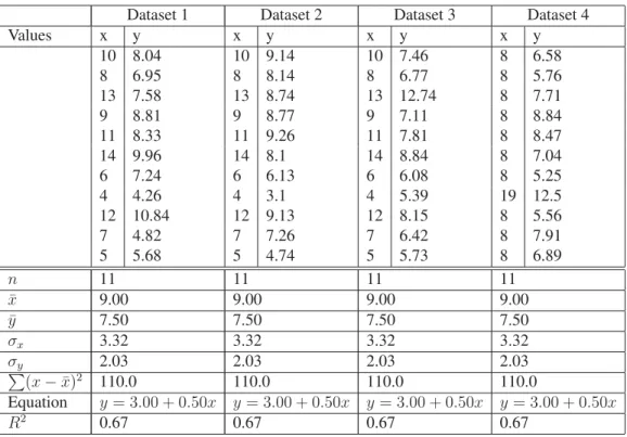
Furthermore, descriptive statistics are sometimes insufficient to understand the details present in data. Anscombe (1973) presents the four data sets shown in Table 1.1 that appear identical under cursory analysis — each having equal averagesx¯andy¯, standard deviations σxandσy,
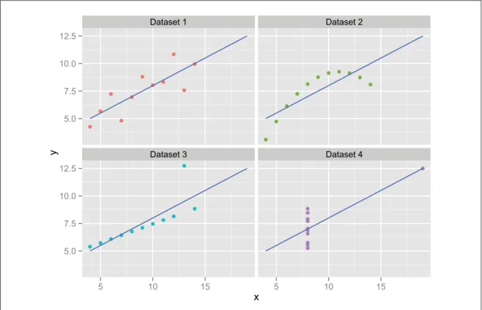
as well as the same linear regression equation and correlation coefficient R2 — yet are very different when displayed graphically, as in Figure 1.1. Anscombe (1973) makes the case that one should not only rely on statistical analysis but should also visualize the data in order to understand it.
Table 1.1 Data for Anscombe’s Quartet: four different data sets of(x, y)points that nevertheless share the same summary statistics.
Dataset 1 Dataset 2 Dataset 3 Dataset 4
Values x y x y x y x y 10 8.04 10 9.14 10 7.46 8 6.58 8 6.95 8 8.14 8 6.77 8 5.76 13 7.58 13 8.74 13 12.74 8 7.71 9 8.81 9 8.77 9 7.11 8 8.84 11 8.33 11 9.26 11 7.81 8 8.47 14 9.96 14 8.1 14 8.84 8 7.04 6 7.24 6 6.13 6 6.08 8 5.25 4 4.26 4 3.1 4 5.39 19 12.5 12 10.84 12 9.13 12 8.15 8 5.56 7 4.82 7 7.26 7 6.42 8 7.91 5 5.68 5 4.74 5 5.73 8 6.89 n 11 11 11 11 ¯ x 9.00 9.00 9.00 9.00 ¯ y 7.50 7.50 7.50 7.50 σx 3.32 3.32 3.32 3.32 σy 2.03 2.03 2.03 2.03 (x−x¯)2 110.0 110.0 110.0 110.0 Equation y= 3.00 + 0.50x y= 3.00 + 0.50x y= 3.00 + 0.50x y= 3.00 + 0.50x R2 0.67 0.67 0.67 0.67
Ware (2004) explains that data visualization provides an ability to comprehend huge amounts of data by using the perceptual power of the brain’s visual processing system. Tory and Möller (2004b) add that by using the advantages of visual perception, we can compensate for cogni-tive barriers, such as a limited working memory. Table 2.2 of Thomas and Cook (2005) lists additional advantages of visualization.
7 ● ● ● ● ● ● ● ● ● ● ● ● ● ● ● ● ● ● ● ● ● ● ● ● ● ● ● ● ● ● ● ● ● ● ● ● ● ● ● ● ● ● ● ● Dataset 1 Dataset 2 Dataset 3 Dataset 4 5.0 7.5 10.0 12.5 5.0 7.5 10.0 12.5 5 10 15 5 10 15 x y
Figure 1.1 Plot of Anscombe’s Quartet: visualizing the data shows large differences between datasets. The linear regression is shown in blue.
1.2 Business intelligence technologies
Chaudhuriet al.(2011) give an overview of the various technologies used for business intelli-gence. Typically, business intelligence systems are architected by combining several compo-nents. Operational (also called transactional) databases contain the data used in daily opera-tions. For example, a hypothetical factory that makes nuts and bolts could have an operational database that contains addresses of customers and their orders, while another might contain customer service requests. These databases are collated together during a process called ex-tract, transform and load (ETL), during which the transactional records are extracted from various data sources, transformed into business events suitable for analysis and loaded into a data warehousing system. These data warehouses are often also relational databases, although this need not be. For example, some data warehouse systems use parallel processing systems such as Apache Hadoop when dealing with large data sets.
There are different approaches to querying such data warehouses for analytical purposes. A popular approach, online analytical processing (OLAP) — also frequently called multidimen-sional online analytical processing (MOLAP) — uses structures called data cubes. Data cubes contain precomputed aggregates across sets of predefined dimensions, speeding up certain types of queries. For example, a data cube about sales information for a company with three dimensions (region, quarter and product category) would be as shown in Figure 1.2.
Region East West Central Quar te r Product category Q1 Q2 Q3
Fruit Candy Butter
Figure 1.2 Data cube for a hypothetical supermarket. Each cell of the cube represents an individual aggregate for a particular combination of dimensions.
Each cell of the data cube contains aggregate information about the data matching that partic-ular cell, but not the data itself. This means that certain aggregate operations (COUNT, SUM, MIN, MAX, AVG) can be done in constant time, no matter how much data the cube represents. On large data sets, the cubes might be generated offline during the night, allowing analysts to analyze them the next day.
Wilkinson et al. (2005) mentions an important caveat with the usage of data cubes: because data cubes do not contain the data but only aggregated information about it, several key
statis-9
tics cannot be derived from a data cube, such as the median, mode, percentiles or quartiles. They also do not allow ad hoc queries on dimensions that are not part of the cube. For ex-ample, it is impossible to query the data cube of Figure 1.2 to only show sales by a particular salesman or that have taken place during a particular month, as neither are dimensions of the cube. It would obviously be possible to add more dimensions to the cube to solve this problem, but this also increases the volume of the cube due to dimensional explosion, making it imprac-tical to use cubes with many dimensions. Wilkinsonet al.(2005) summarizes the intersection of data cubes and data visualization in a single sentence: “Few of the graphics in this book and in other important applications can be computed from a data cube.”
On the other hand, the relational online analytical processing (ROLAP) approach stores the data in a relational database and queries it directly; this allows the data to be queried in different fashions as the data is stored verbatim but performance is a function of the amount of data stored in the system.
Because all of these systems are used for business reporting, they compute exact values for any given query. However, for visual analytics, a fast approximation rather than an exact result improves the end user experience, as explored by Fisher et al. (2012). The prototype built by Fisheret al.(2012) builds incremental approximations of a database query, letting the user control the threshold between accuracy and timeliness by waiting for the query to have smaller error bounds. As their prototype was built to explore the user experience of such an incremental visual analytics system rather than designing a high performance incremental query processing engine, it does not address the issue of designing such a system, which is still a current research problem. Later, we will show that VisReduce contributes a new approach for such systems.
1.3 Multidimensional multivariate visualization
Many datasets can be represented in tabular form, with one column for each variable, and one row for each tuple. There are two types of columns: independent variables, also called
dimensions, which are usually categorical variables (or discretized variables that are almost equivalent to categorical variables), anddependent variables, also calledmeasures, which are
normally continuous variables. Such datasets, with a mix of dimensions and measures, are sometimes called multidimensional multivariate, or MDMV, data. Surveys of techniques for visualizing MDMV data can be found in (Wong and Bergeron (1997); Grinsteinet al.(2001); Keim (2002)). We will consider the most relevant of these techniques, and consider a fictitious “bolts” dataset to illustrate some differences between previous work. The nuts-and-bolts data is stored as a table, and involves three (independent) categorical variables: Region (North, Central, or South), Month (January, February, ...), and Product (Nuts or Bolts). It also involves three (dependent) continuous variables: Sales, Equipment costs, and Labor costs. The values of the categorical variables yield3×12×2 = 72combinations of categorical values, each corresponding to a row in a table, and each mapping to values of the continuous variables:
Table 1.2 The tabular representation of the nuts-and-bolts dataset.
Region Month Product Sales Equipment Labor costs costs
North Jan Nuts 2.76 0.92 4.30
North Jan Bolts 4.92 1.64 4.30
North Feb Nuts 4.20 1.00 4.30
North Feb Bolts 8.40 2.00 4.30
North Mar Nuts 5.28 9.60 4.30
..
. ... ... ... ... ...
South Dec Bolts 9.50 2.44 5.20
TableLens (Rao and Card (1994)) and FOCUS (Spenkeet al.(1996)) (later renamed InfoZoom) provide ways to aggregate the tuples in a list such as the one above, while still presenting an essentially tabular view to the user. Both systems allow the user to sort tuples by any variable, but have limited ability to ease the understanding of multiple categorical variables.
Scatterplot matrices (SPLOMs) were proposed by Hartigan (1975), and display a scatterplot for every possible pair of variables. Notable more recent work includes Scagnostics (Wilkinson
11
et al.(2005)), which enable SPLOMs to scale up to many continuous variables, and Scatter-dice (Elmqvist et al. (2008)), which demonstrates how they can be made highly interactive. SPLOMs nevertheless have shortcomings when used to visualize categorical variables. In Fig-ure 1.3, the top three scatterplots (e.g., Month vs Region) each show a crossing of two categor-ical variables, resulting in an uninformative grid of points. Scatterplots showing a continuous vs categorical variable suffer from overplotting: in the Sales vs Product scatterplot, it is not obvious which of the products resulted in higher overall sales.
Figure 1.3 A SPLOM of the nuts-and-bolts dataset.
HyperSlice (van Wijk and van Liere (1993)) displays a matrix of slices of a scalar function of many dimensions, but cannot display several (dependent) continuous variables at once. The heatmaps of GPLOM, explained in the next chapter, are similar to HyperSlice, though GPLOM’s heatmaps display aggregations of data rather than slices.
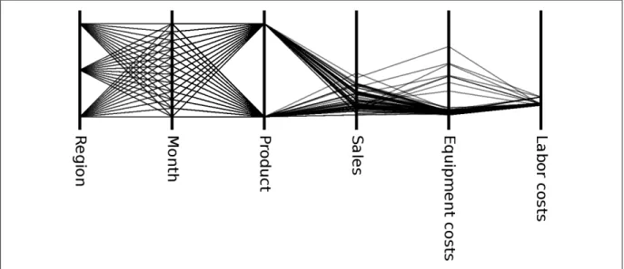
Parallel coordinates (Inselberg (1985); Wegman (1990)) show each tuple as a polygonal line intersecting an axis once for each of the variables. Figure 1.4 shows an example. The 3 right-most axes show continuous variables, allowing us to see the distribution of values along them (the range and central tendency of values, and outliers). However, the three left-most axes show categorical variables, where every possible combination of values is covered, resembling complete bipartite graphs. This creates ambiguities that prevent us from visually tracing a tuple across all axes (although interactive highlighting could alleviate this).
A technique called parallel sets (Bendixet al.(2005)) displays multiple categorical variables side by side, as in a parallel coordinate plot. While it allows tracing tuples across multiple axes, parallel sets also have very cluttered displays when used with high cardinality variables.
Figure 1.4 A parallel coordinates plot of the nuts-and-bolts dataset.
Various combinations of scatterplots and parallel coordinates have been proposed, displaying them side-by-side (Quet al.(2007); Steedet al.(2009)) or more tightly integrated (Yuanet al.
(2009); Holten and van Wijk (2010); Viauet al. (2010); Claessen and van Wijk (2011)), but none of these approaches facilitate the visualization of categorical variables.
Arrays of glyphs can be used to visualize MDMV data, where each glyph shows one tuple (Bertin (1967); Chernoff (1973); Kleiner and Hartigan (1981); Pickett and Grinstein (1988);
13
Ward (2002)). This works well when there are at most 2 (independent) categorical variables. For example, an arrow plot (Wittenbrinket al. (1996)) can display an arrow-shaped glyph at each of the points on a 2D grid, showing wind speed and wind direction over a geographic map. Extending this to 3 spatial dimensions results in occlusion, and beyond 3 dimensions it becomes very difficult to understand the ordering of glyphs along each dimension.
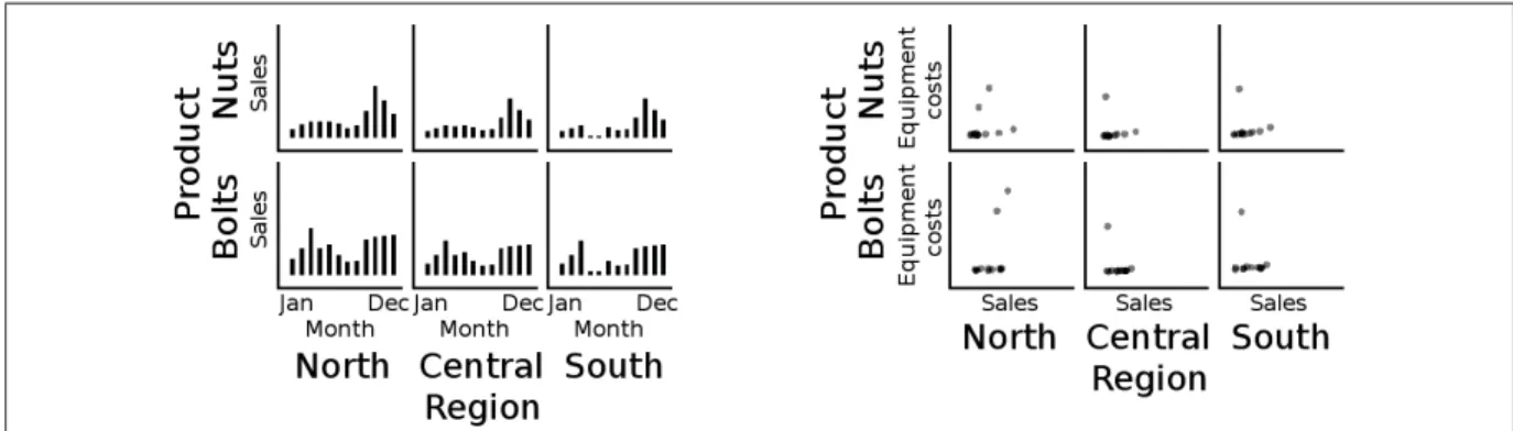
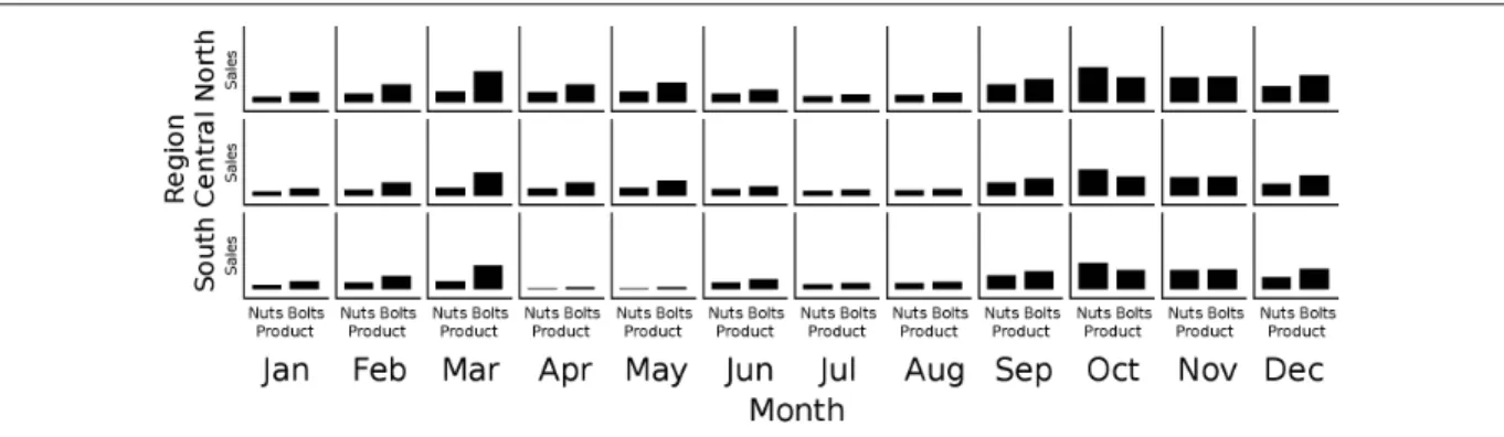
Dimensional stacking (LeBlanc et al. (1990); Mihalisinet al. (1991)) allows more than one categorical variable to be mapped to the same spatial axis, and has been used in database visu-alization (Stolteet al.(2002a); Mackinlayet al.(2007)). Figures 1.5 and 1.6 show examples, each of which shows a total of 4 variables. The two innermost variables of the stacking de-termine the type of chart shown: if the innermost vertical variable is a continuous variable (e.g., Sales), and the innermost horizontal variable is a categorical variable (e.g., Month), then barcharts are used. On the other hand, scatterplots are used if the two innermost variables are continuous variables (e.g., Equipment costs vs Sales).
Figure 1.5 Examples of dimensional stacking with the nuts-and-bolts data. Left: Product and Sales are mapped to the vertical axis, Region and Month are mapped to the horizontal. Right: Product and Equipment costs mapped to the vertical, Region and Sales
to the horizontal.
Each of the charts in Figures 1.5 and 1.6 show asliceof the data, allowing the user to see more detail. For example, Figure 1.6 reveals that sales were very low in the South in April and May. By comparison, in Figure 1.3, the Sales vs Month scatterplot also shows low sales in April and May, without revealing the Region.
Figure 1.6 Another example of dimensional stacking applied to the nuts-and-bolts data. Region and Sales are mapped to the vertical axis, Month and Product to the horizontal. The added detail visible in Figures 1.5 and 1.6, however, comes at the cost of exponential growth in space requirements as categorical variables are added. For example, if the dataset had an additional categorical variable Year with values 2001, 2002, ..., 2010, adding this as an outer variable to Figure 1.6 would increase the number of charts by a factor of 10. Partly for this reason, software like Tableau (Mackinlayet al.(2007)) does not show the user an initial visualization of the data. Instead, Tableau initially shows a list of variables (Figure 1.7) from which the user may drag and drop to construct a desired visualization (Figure 1.8).
Figure 1.7 An empty workbook in Tableau. At this point, the user must construct a visualization by dragging variables onto the shelves. Tableau’s interface does not expose
15
Figure 1.8 A visualization in Tableau. In this case, the user has added several filters to see a subset of the data and built a visualization that shows the median of a variable,
broken down by state.
Figure 1.9 A generalized pairs plot generated with theggpairspackage, showing all pairs of dimensions. Plot types in this pairs plot are — from top left to bottom right — bar
charts of variable cardinality, box plots of variable distribution, barcode plots of variable distribution, scatterplots and correlation coefficients.
Emerson et al. (2013) propose the generalized pairs plot (Figure 1.9), which extends the SPLOM by using different types of charts depending on the types of variables paired together, alleviating the problems that occur when categorical variables are shown in a SPLOM (Fig-ure 1.3). The generalized pairs plot is promising step in the direction of better visualizations of multidimensional multivariate datasets, because the choice of chart in the matrix is based on the types of variables involved. However, Emerson et al.(2013)’s work still leaves room for improvement. First, their implementation only generates static visualizations. Many interac-tive features could be added, to allow the user to interacinterac-tively highlight and explore the data in the visualization. Second, their implementation uses several kinds of charts, some of which (such as mosaic plots and boxplots) do not scale well for high-cardinality variables and may
be unfamiliar to casual business users. We therefore propose the GPLOM (Generalized PLOt Matrix) that makes Emerson et al. (2013)’s generalized pairs matrix both highly interactive, and simpler to understand.
CHAPTER 2
THE GENERALIZED PLOT MATRIX
2.1 Introduction
Many datasets are stored in tabular form, with one row for each tuple, and one column for each attribute. If the attributes aredependent variables(e.g., dependent variables of a key or row id), we speak ofmultivariatedata, for which many techniques exist for visualizing several variables at once, such as scatterplot matrices (SPLOMs) (Hartigan (1975)), parallel coordinates (Insel-berg (1985)), and glyphs (Bertin (1967); Chernoff (1973); Kleiner and Hartigan (1981); Pickett and Grinstein (1988)). Some of the columns, however, may be best thought of asindependent variables, in which case we speak of multidimensional multivariate (MDMV) data (Wong and Bergeron (1997)). Stolteet al. (2002a) use the term dimensionfor a (categorical or ordinal) independent variable, and measure for a dependent variable. We will refer to dimensions as categorical variables, and measures as continuous variables.
The aforementioned techniques, of SPLOMs, parallel coordinates, and glyphs, all suffer from problems when naively applied to datasets with many categorical variables. An alternative approach involves “stacking” multiple categorical variables along axes, used in trellis charts and other techniques (LeBlanc et al. (1990); Mihalisin et al. (1991); Stolte et al. (2002a)) and more recently in the commercially successful product Tableau (Mackinlayet al.(2007)). However, dimensional stacking suffers from a combinatorial explosion if too many categorical variables are displayed at once.
Recent work (Emersonet al.(2013)) offers a new solution for visualizing MDMV data, based on the observation that SPLOMs need not display scatterplots for all pairs of variables. A plot matrix could instead display different charts for different pairs of variables, which Emerson
et al.(2013) demonstrated with a wide variety of charts. We adapted this idea with our own technique called the Generalized Plot Matrix (GPLOM). In our approach, the visualization is simpler than Emerson et al. (2013)’s, as we use only three kinds of charts, chosen with
rules similar to those of Mackinlayet al.(2007): scatterplots for pairs of continuous variables, barcharts to show a continuous variable as a function of a categorical variable, and heatmaps to show a selected continuous variable as a function of a pair of categorical variables. These three charts are the minimum number necessary to cover the three possible pairings of variable types. This makes the matrix easier to understand, which could be beneficial to casual business users and other non-expert users. At the same time, we extend part of Emersonet al.(2013)’s work by presenting interactive features for highlighting, selecting, searching, and filtering the data.
Both Emersonet al.(2013)’s technique, and our own GPLOM, can comfortably display sev-eral categorical and continuous variables at once, avoiding the combinatorial explosion of di-mensional stacking because the data can be aggregated within each chart. This makes these approaches appropriate for data with multiple categorical variables, as is common in business intelligence and other domains. These approaches can also provide the initial overview of a database shown to a user, serving as a visual launching point for further investigation. This is in contrast to the approach in Polaris (Stolte et al.(2002a)) or Tableau (Mackinlay et al.
(2007)), where the user must first select one or several variables of interest to explicitly con-struct a visualization. Finally, for non-expert users, the GPLOM approach has the advantage of only using three kinds of charts, avoiding the more complicated charts such as mosaic plots or box plots that may be difficult for non-expert users to understand and that don’t scale as well to high cardinality variables.
Our contributions in this chapter are (1) the GPLOM technique for visualizing multidimen-sional multivariate data using only three kinds of charts, making it as easy to understand as possible while still showing charts that are adapted to the kinds of variables involved; (2) a de-scription of the visual design choices and features of our prototype implementation, including bendy highlights, associative highlighting, and a text search feature that highlights data, allow-ing users to quickly find charts of interest; and (3) an experimental comparison of GPLOM and Tableau that found GPLOM to be significantly faster in certain cases.
19
2.2 Previous Work
The most closely related work to ours is the Generalized Pairs Plot (Emerson et al. (2013)), which extends the matrix in a SPLOM to allow a mix of chart types to be displayed, including mosaic plots, box plots, histograms, and density contours. As demonstrated in the next sec-tion, this is scalable to a larger number of continuousandcategorical variables than previous techniques, because the space requirements scale linearly with the number of variables, rather than exponentially as with the previous example of dimensional stacking. Our GPLOM work further explores Emerson et al.’s ideas by (1) only using three kinds of charts, to make the visualization easier to understand by non-expert users who may simply want a visual overview of a business database as a first step in asking analytic questions; and by (2) extending the static plots of Emerson et al. (2013) through interactive techniques. We also (3) empirically compared GPLOM to a commercial product and found significant advantages with GPLOM in certain cases.
2.3 Description
Figure 2.1 shows an example GPLOM of 6 variables. In the Sales vs Product chart, we clearly see that Bolts outsold Nuts, thanks to the use of aggregation (via a sum operator) that generated the bar heights. The overplotting seen in Figure 1.3’s Sales vs Product scatterplot is thus avoided.
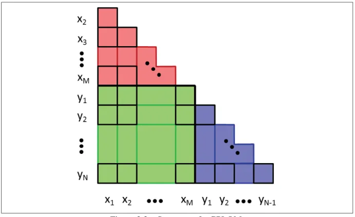
Figure 2.2 shows the layout of a GPLOM for M categorical variablesx1, ..., xM and N
con-tinuous variablesy1, ..., yN. A full matrix would have (M +N)×(M +N)cells, however
we only display the lower triangular half, without the diagonal, as is often done with SPLOMs (e.g., Wilkinsonet al.(2005)). Thus, our GPLOM saves space compared to the full matrices of Emersonet al.(2013), leaving room for interactive elements such as the infobox (discussed shortly).
The red region in Figure 2.2 contains pairs of categorical variables, and GPLOM visualizes these with heatmaps. The green region contains pairings of a continuous vs categorical vari-able, shown as barcharts. The purple region contains pairs of continuous variables, shown as
Figure 2.1 A GPLOM of the nuts-and-bolts dataset. Barcharts and heatmaps show data aggregated by sum. The vertical axes on the barcharts extend to 250, to accommodate the
larger values than in the scatterplots. The heatmaps are colored to show “Sales” as a function of categorical variables, and use a color scale varying from cyan for low values,
through grey for mid values, to red for the highest values.
scatterplots. (This grouping of variable types is comparable to Penget al.(2004)’s ordering of variables in a SPLOM according to their cardinality.) Note that the scatterplots show individual tuples, whereas the barcharts and heatmaps show aggregated data.
Other charts in these regions are possible, as demonstrated by Emerson et al.(2013), such as boxplots or linecharts. However, their example plots show categorical variables with at most four distinct values. Complex charts, such as box plots and mosaic plots, become difficult to read with categorical variables with high-cardinality (Figure 2.3).
An interactive prototype of the GPLOM technique was created using D3 (Bostocket al.(2011)) and JavaScript. Figure 2.4 shows the prototype displaying a large real-world dataset, where the categorical variables of Year, Day of month, and Carrier have 26, 31, and 32 distinct values,
21
Figure 2.2 Structure of a GPLOM.
respectively. As can be seen in Figure 2.4, restricting the GPLOM to only show three kinds of simple charts — heatmaps, barcharts, and scatterplots — helps keep the charts readable at these higher cardinality values.
One tradeoff in designing a GPLOM is deciding if axes of the same variable should be scaled to the same range (facilitating comparisons of adjacent charts) or scaled to the maximum of the data in the chart. In Figure 1.3, all axes are scaled to 35. However, in Figure 2.1, the barcharts contain (aggregated) sums, and are therefore scaled to a larger range. The scatterplots in Figure 2.1, however, are still scaled to 35, to avoid having all the points clustered in a corner of the scatterplots. Furthermore, the heatmaps in Figure 2.1 share the same color scale, and we notice that only one of the heatmaps has a value close to the maximal red, because the other heatmaps are subdivided into months, reducing the values in them. Figure 2.4 instead scales each chart independently, according to the maximal value within it. This makes better use of spatial (and color) resolution, but makes it more difficult to compare charts.
Figure 2.3 Example plots extracted from a matrix generated with thegpairspackage in R (Emerson and Green (2012)). Top row: boxplots over variables of cardinality 5, 13, and 35, respectively. Bottom row: mosaic plots with cardinality 3×5, 5×13, and 13×35,
respectively.
2.3.1 Interaction
The user may interact with the GPLOM in several ways. A GPLOM contains bars and rectan-gles that afford easier pointing and clicking than the small points or dots in a normal SPLOM. In our GPLOM prototype, rolling the mouse cursor over a barchart bar or heatmap cell causes it to highlight. Clicking on a bar or cell selects it.
2.3.1.1 Linking
Linking (or coordination (Roberts (2007); Wang Baldonadoet al.(2000); North and Shneider-man (2000))) between charts is shown in two ways: bendy highlights, and associative high-lighting.
Bendy highlights are specialized links that connect different charts, comparable to previous work that also draw links between views (Collins and Carpendale (2007); Steinberger et al.
(2011); Claessen and van Wijk (2011); Viau and McGuffin (2012)). Bendy highlights are curved links that show the value of a categorical variable during rollover or selection. A text
23
Figure 2.4 A GPLOM of 8 categorical variables, 8 continuous variables, and 144 million flights from the OnTime dataset. The menubar at the top displays the possible aggregation operators for barcharts and heatmaps: Average (currently selected), Sum, Count, Min, and Max. The menubar also shows that “Departure delay” is the currently
selected (dependent) continuous variable for heatmaps. Other interface elements: A: bendy highlight; B: textual search box; C: infobox. Note that heatmaps and barcharts are computed over the whole dataset, but scatterplots only show a random sample of 200 data
points each.
string is displayed at the curved corner of the link to show the category (for example, the 5-6pm departure time block is displayed as “1700-1759” on the corner of the bendy highlight in Figure 2.4, A). Bendy highlights can also help understand the relationship between a heatmap cell and other charts (Figure 2.5).
Associative highlighting shows the relationship between charts when a categorical value is se-lected. There are three types of such highlighting. If the aggregation used in barcharts and heatmaps is the Sum or Count operator, then associative highlighting is achieved by highlight-ing the fraction of bars in other barcharts that is associated with the selected value (Figure 2.6). This is similar to the proportional highlighting of bars of Zhang and Marchionini (2004). If, in-stead, the aggregation used is Average, Min, or Max, then associative highlighting is achieved
Figure 2.5 Bendy highlights and a tooltip.
by displaying dots to show the average, min, or max value of data for the selected value (Fig-ure 2.7). Finally, regardless of the aggregation operator, the corresponding dots in the scatter-plots are highlighted.
2.3.1.2 Filtering
To drill down, the user can double click on a bar (such as a bar for “Year” = 2012), causing a filter to be created that restricts the displayed data to that value. This “sheds” the corresponding categorical variable, removing a row and column of charts from the GPLOM, and creates a filter box that the user can later click on to roll back up. Figure 2.6 shows the result of applying four successive filters: “Year” = 2012, “Quarter” = 1, “Month” = 1 and “Carrier” = EV. We call this feature “dimensional shedding”.
2.3.1.3 Infobox
Additional information about the element under the cursor is displayed in the infobox (upper right corner of Figure 2.4), which contains the results of the various aggregation operators
25
Figure 2.6 With the Sum aggregation operator, associative highlighting fills in the fraction of bars associated with the selected value “Departure time block” = “1800-1859”.
Figure 2.7 With the average aggregation operator, associative highlighting displays circles showing the average values for the selected value “Departure time block” =
“1800-1859”.
as well as a kernel density estimate plot, allowing the user to judge whether the underlying distribution is normal or not, its modality and its skewness.
2.3.1.4 Text Search
Because GPLOM displays a large number of charts, it may be time consuming for users to visu-ally scan all variable names to find a desired chart. Thus, a textual search function (Figure 2.8) allows the user to enter a string, suggests autocompletions, and highlights the corresponding elements once the string is entered. Currently, our prototype only allows the user to enter val-ues, however it would be easy to extend the prototype to also allow entering names of variables. This feature is similar to one proposed in section 6.1 of Grammelet al.(2010).
Figure 2.8 Entering the name of a value causes it to be highlighted in the GPLOM.
2.3.1.5 Labels
Due to the density of information displayed in a typical GPLOM, there is often insufficient room for labels showing the values of all categorical variables along their axes. Instead, GPLOM relies heavily on tooltips and bendy highlights that show the value under the cur-sor. In our first version of the prototype, we arranged categorical values on vertical axes sorted top-to-bottom, resulting in Figure 2.9. This resulted in many crossing bendy highlights. We therefore modified the prototype to sort values bottom-to-top, yielding Figure 2.10, which is the order shown in other figures in this paper. A third possibility is shown in Figure 2.11, which avoids excessive crossed links while maintaining the usual top-to-bottom ordering of values.
27
Figure 2.9 A variant of bendy highlights: alphabetical vertical sorting (e.g., Asia, Europe, USA).
Figure 2.10 A variant of bendy highlights: reverse alphabetical vertical sorting (e.g., USA, Europe, Asia).
Figure 2.11 A variant of bendy highlights: a “reversed” GPLOM with alphabetical vertical sorting.
2.4 Implementation
The GPLOM architecture follows the three-tier architecture. The data tier is a standard SQL database such as SAP HANA or MySQL, the logic tier consists of a web application imple-mented using the Play framework1 and the presentation tier is a JavaScript application that renders SVG on the client’s browser using D3.
The logic tier computes aggregates as requested by the presentation tier and serves as an ab-straction of the underlying database.
2.5 Experimental Evaluation
We suspect that one of the advantages of GPLOM is that users can answer questions by sim-ply scanning for the appropriate chart, whereas in the commercial product Tableau they must explicitly construct a visualization. To investigate this idea, we performed an experimental comparison of user performance with both tools.
29
We chose three datasets for the experiment: a warm-up dataset (a converted sample SQL server database called Adventureworks) that was used to introduce users to both visualization tools, and two other datasets (Cars2, and the OnTime3 airline delay data for the month of December 2012). Cars and OnTime were each used with one of the tools, counterbalanced for dataset and ordering. One quarter of the users did (Tableau+Cars, GPLOM+OnTime), another quarter did (Tableau+OnTime, GPLOM+Cars), another quarter did (GPLOM+OnTime, Tableau+Cars) and the last quarter did (GPLOM+Cars, Tableau+OnTime).
Each trial required the user to answer a question about the dataset. There were two types of questions, and for each type of question, there could be zero or more criteria involved in the question. Thetype of questionconsisted of either questions that asked which type of trend or correlation (positive, negative or null) exists between two variables, if any, and questions that asked to find a particular data value, such as the year in which the average mileage per gallon for all cars was the highest. The criteria count ranged between zero to three criteria, so that a question “find the carrier with the highest average arrival delay” has zero criteria, while the question “find the day of the week when Hawaiian Airlines (HA) has the highest average delay for flights departing between 9:00-9:59” has two criteria (carrier=HA, departureTime=0900-0959).
In total, the experiment involved: 2 types of questions (trend or data)
×4 criteria counts (0 through 3)
×2 technique-dataset pairs (GPLOM and Tableau 7.0)
×12 users = 192 trials
The 12 students who participated (11 male, 1 female) were either from the software engineer-ing or information technology engineerengineer-ing programs at ETS, at both the undergraduate and graduate levels. Each student was assigned to one of the four between-subjects groups and was
2http://lib.stat.cmu.edu/datasets/
asked to explore the warm-up dataset for five minutes with one of the two techniques (either Tableau or GPLOM, depending on the participant’s group), as an exploration phase. Once the five minutes were over, each participant was shown how to use the software in order to answer the questions, then presented with eight questions for the warm-up dataset. After the questions on the warm-up dataset were answered, a second dataset (either Cars or OnTime, depending on the participant’s group) was shown and the participant was asked to answer questions about the new dataset. Then, the participant explored the warm-up dataset again, using the other technique, answered the same eight questions using the other technique and, finally, answered a set of questions on a different dataset than the one explored with the first technique.
None of the participants indicated that they had any prior experience with Tableau or with the GPLOM prototype. During the exploration phases and warm up trials, users were free to ask questions, and were shown all the features of the user interfaces that were necessary to answer the questions in the experiment.
The participants used a single monitor workstation equipped with a 24 inch monitor, keyboard and mouse.
The GPLOM prototype consisted of a web application built using D3 and JavaScript, running in the Chrome web browser (version 25), as well as a server-side backend. The server-side backend managed communication between the client and a MySQL server, computing agre-gates to be consumed by D3. It was built using the Play framework 2.0.4 and ran in production mode during user tests.
Tableau and GPLOM both connected to the same MySQL database over a wired gigabit Eth-ernet network.
As the GPLOM prototype was not optimized for performance, each time a participant added a filter by double clicking, a full page load by Chrome was executed, requiring Chrome to re-interpret and run JavaScript code (in theory, this could be eliminated with more careful coding) and also regenerating all charts (this is unavoidable with the GPLOM approach). We
31
subsequently measured that the median time for all this to occur was 1.7 seconds for the Cars dataset, and 5.7 seconds for OnTime.
The questions were displayed to users on a second monitor controlled by the experimenter. When the user indicated they were ready to start a trial, the experimenter clicked a button to display the question and start a timer. The user then read the question and interacted with the vi-sualization tool until they said they could answer the question, at which point the experimenter stopped the timer (triggering a simultaneous screen grab of the user’s screen), and transcribed the user’s verbal answer. The time elapsed was recorded. If the user decided they wished to check or change their answer by performing further interactions with the visualization tool, the time of their last answer determined the recorded duration. No feedback was given to indicate to the user if their final answer was correct or incorrect.
2.5.1 Results
Because each participant was only exposed to half of the four {GPLOM, Tableau}× {Cars, OnTime} combinations, the performance data were separated by dataset for analysis. Some of the main results are summarized in Figure 2.12 and below:
Table 2.1 Breakdown of error rate and median time to complete tasks by dataset and technique.
GPLOM Tableau
median time (s) error rate median time (s) error rate
Cars 23.67 13% 41.14 10%
OnTime 48.68 17% 59.58 33%
The time taken by participants to answer was non-normally distributed (Shapiro-Wilk normal-ity test, p < 0.01). The non-parametric ANOVA-type statistic (ATS) revealed that GPLOM was significantly faster than Tableau for the Cars dataset (p <0.01), and that the criteria count had a significant effect on time in both the Cars dataset (p < 0.01) and the OnTime dataset