Sampling and Subspace Methods for Learning Sparse Group Structures in Computer Vision

(1)

University of Central Florida University of Central Florida

STARS

Electronic Theses and Dissertations, 2004-2019

2018

Sampling and Subspace Methods for Learning Sparse Group

Structures in Computer Vision

Maryam Jaberi

University of Central Florida

Part of the Computer Sciences Commons

Find similar works at: https://stars.library.ucf.edu/etd University of Central Florida Libraries http://library.ucf.edu

This Doctoral Dissertation (Open Access) is brought to you for free and open access by STARS. It has been accepted for inclusion in Electronic Theses and Dissertations, 2004-2019 by an authorized administrator of STARS. For more information, please contact [email protected].

STARS Citation STARS Citation

Jaberi, Maryam, "Sampling and Subspace Methods for Learning Sparse Group Structures in Computer Vision" (2018). Electronic Theses and Dissertations, 2004-2019. 5791.

(2)

SAMPLING AND SUBSPACE METHODS FOR LEARNING SPARSE GROUP STRUCTURES IN COMPUTER VISION

by

MARYAM JABERI

M.S. University of Nevada Reno, 2012

A dissertation submitted in partial fulfilment of the requirements for the degree of Doctor of Philosophy

in the Department of Computer Science

in the College of Engineering and Computer Sciences at the University of Central Florida

Orlando, Florida

Spring Term 2018

(3)

c

(4)

ABSTRACT

The unprecedented growth of data in volume and dimension has led to an increased number of computationally-demanding and data-driven decision-making methods in many disciplines, such as computer vision, genomics, finance, etc. Research on big data aims to understand and describe trends in massive volumes of high-dimensional data. High volume and dimension are the deter-mining factors in both computational and time complexity of algorithms. The challenge grows when the data are formed of the union of group-structures of different dimensions embedded in a high-dimensional ambient space. To address the problem of high volume, we propose a sampling method referred to as the Sparse Withdrawal of Inliers in a First Trial (SWIFT), which determines the smallest sample size in one grab so that all group-structures are adequately represented and dis-covered with high probability. The key features of SWIFT are: (i) sparsity, which is independent of the population size; (ii) no prior knowledge of the distribution of data, or the number of underlying group-structures; and (iii) robustness in the presence of an overwhelming number of outliers. We report a comprehensive study of the proposed sampling method in terms of accuracy, functionality, and effectiveness in reducing the computational cost in various applications of computer vision. In the second part of this dissertation, we study dimensionality reduction for multi-structural data. We propose a probabilistic subspace clustering method that unifies soft- and hard-clustering in a single framework. This is achieved by introducing a delayed association of uncertain points to subspaces of lower dimensions based on a confidence measure. Delayed association yields higher accuracy in clustering subspaces that have ambiguities, i.e. due to intersections and high-level of outliers/noise, and hence leads to more accurate self-representation of underlying subspaces. Alto-gether, this dissertation addresses the key theoretical and practically issues of size and dimension in big data analysis.

(5)

To my mom and dad

(6)

ACKNOWLEDGMENTS

Over the past six years, I have received support and encouragement from numerous individuals. First, I would like to thank my doctoral adviser, Dr. Hassan Foroosh, for his invaluable insights and much-needed support. His guidance has made this a thoughtful and rewarding journey. I would also like to thank my doctoral co-adviser, Dr. Marianna Pensky, for her friendly guidance, thought provoking suggestions, and many valuable contributions. My sincere appreciation is extended to the members of my dissertation committee, Dr. Guo-Jun Qi and Dr. Boqing Gong. Their contribution was crucial to a timely completion of this dissertation. I owe many thanks to Jussi Doherty for his encouragement and hours of proofreading. My most heartfelt gratitude is for my parents and my sisters, whose love and guidance are with me in all my pursuits.

(7)

LIST OF FIGURES

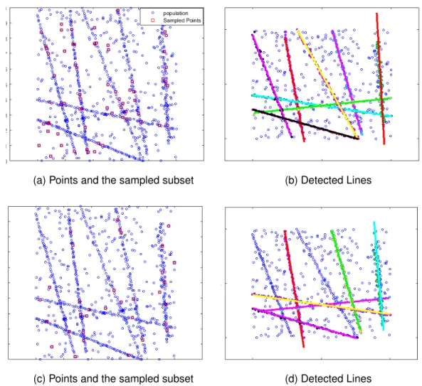
Figure 3.1: The population includes 8 lines and50%gross outliers. (a): shows the data points and sampled subset when the size of the sample set is calculated using SWIFT. (b) shows the detected lines using SWIFT samples and mean-shift. (c) and (d) show the underestimated sample size and the detected lines, failing to find all the instances in the data. . . 33

Figure 3.2: Comparison of estimatedraveraged over 200 independent trials versus ground-truth ofrwhenN ∈ {103_,₁₀4_,₁₀5_}_,_ε_{∈ {}₂_,₅_}_and_C _{∈ {}₅_,₅₀_}_{. . . .} ₃₅

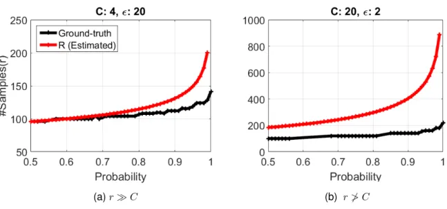
Figure 3.3: Examine the average accuracy of estimated r using multinomial estimation in (3.18). HereN = 105 _{and from left to right}_ε₌_{₂₀_,₂_}_and_C _{∈ {}₄_,₂₀_}_.

The condition ofrCis satisfied in (a) and violated in (b) . . . 36

Figure 3.4: Estimated values of lower bound and upper bound ofrfor1−δaveraged over 200 independent trials versus the ground-truth when N = 104 _and _ε _{= 4}_.

From left to right:C ∈ {5,20,50}. . . 37

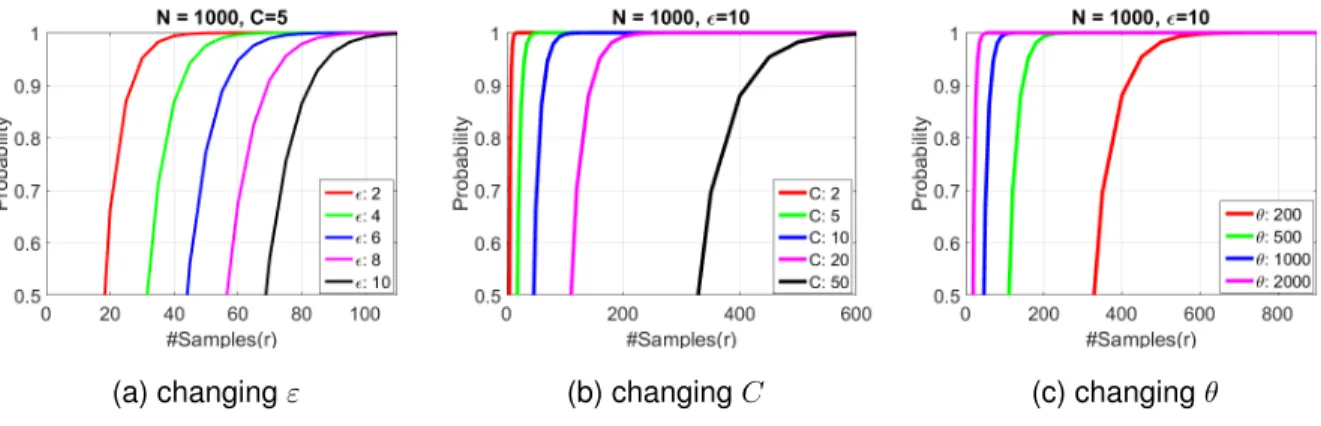
Figure 3.5: The effect of changing different parameters on the sample size r. (a): In-creasing the value ofεforces the method to select more samples in order to remain with the same probability. (b) and (c): increasingC or decreasingθ forces the method to grab more samples to reach the same probability. . . 39

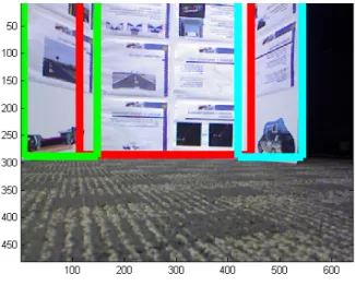
Figure 3.6: Using SWIFT to detect 3D Planes when 1 − δ = 0.9 (a): Data is from Castelvecchio dataset [79] where r = 42 and N = 754. (b): Blue points are outliers that are not grouped in any model whenr= 43andN = 3000. . . 42

(12)

Figure 3.7: Detecting planes in 3D point cloud data collected using a Kinect. . . 43

Figure 3.8: Synthetic data for multibody structure from motion. The outliers are added after moving objects and computing the 2D projections. These outliers are not shown in this figure. (a): The 3D objects that are not necessarily planar. (b): 3D objects are moved randomly and independently. (c): The image is taken from (a). (d): The image is taken from (b) after moving the camera. . . 45

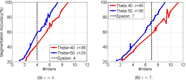
Figure 3.9: The effect of changing percentage of outliers on required sampled points and accuracy of multibody structure form motion in [72]. The results are in the presence of 3 independent motions and when the image segmentation has an average accuracy of 65%and θ = 40. (a): %of Detected models. (b), (c): Values of r when ε = {4,7} respectively. (d): initial candidates for both homographies and fundamental matrices. . . 47

Figure 3.10: The effect of image segmentation accuracy on the average number of inliers sampled in each model instance when we have three motions. . . 48

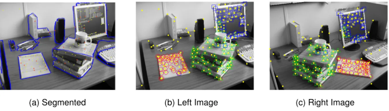
Figure 3.11: Detecting multibody structure from motion when the segmentation accu-racy is 80% and N = 200 includes 25% gross outliers. For fundamental matrices, the sample sizes arer = 63andr = 50for multinomial and hyper-geometric models, respectively. (a): segmented image. Yellow dots are the correspondences, and red stars are the sampled points using SWIFT. (b),(c): images with 3 objects moved independently and the detected motions using the method in [72]. . . 49

(13)

Figure 3.12: Comparing the averaged number of samplesrover 200 trials in sequential RANSAC, the proposed method (MBSAC) in [33], and SWIFT whenN = {102,103,104},ε= 2andP = 0.9. . . 51

Figure 4.1: The effect of changing the ratio of inliers (ρ) on accuracy of clustering. The estimated SWIFT sample size when 1−δ = 0.9 is shown in gray dotted lines. Whenρ= 3, the actual size of the sampled population needs to be225 (ground truth), the calculated value by SWIFT sampling using hypergeomet-ric and multinomial pmf models are193and219, respectively. These results were averaged over100trials. . . 56

Figure 4.2: Example of Images in the Extended Yale B Database. . . 59

Figure 4.3: Accuracy of clustering face images. Computed SWIFT sample sizes using both multinomial and hypergeometric estimations are shown in gray lines. In this experiment,N = 320, P = 0.9, andC = 5. Results are averaged over 100images. . . 60

Figure 5.1: Affinity between different subspaces coded in matrix M when there are 3 subspaces. . . 73

Figure 5.2: Updates inΩover10iterations for3different cases of2,3and4classes and 50%intersection. . . 74

Figure 5.3: Updates inΩover10iterations for3different cases of2,3and4classes and 70%intersection. . . 75

(14)

Figure 5.4: Updates in A (top) and Z¯ (bottom) over two consecutive iterations. Data includes3subjects and70%intersection. . . 77

Figure 5.5: Average%misclassification errors (5.10) for Prob-SSC, SSC and S3C meth-ods over20independent trials. . . 81

Figure 5.6: Average%misclassification errors over 10 iterations. Results are shown for Prob-SSC, SSC and S3C. . . 82

Figure 5.7: Average decrease of%uncertainpoints. . . 82

Figure 5.8: Average%misclassification errors for points that are not falling on the inter-section of subspaces. . . 84

Figure 5.9: Sample images in YaleB Dataset . . . 85

Figure 5.10: Updates inA(top) andZ¯ (bottom) over three consecutive iterations. Data is from the Yale B Face Dataset with5subjects. The misclassification errors are7.19%,1.25%and1.0%in iterationst={1,2,3}respectively. . . 86

Figure 5.11: Images from the Hopkins 155 dataset. . . 88

Figure 5.12: Updates in A (top) and Z¯ (bottom). Data is from the Hopkins155 with 2 subjects. The percentage of uncertain points ar 10%, 2% and 0.0% and misclassification errors are 2.42%, 1.93% and 0.48% in iterations {1,2,4}

(15)

LIST OF TABLES

Table 3.1: Performance comparison among 3 different scenarios of (i) SWIFT sample size (ii) underestimated sample size (iii) overestimated sample size. . . 41

Table 4.1: Comparing the size of SWIFT sampling, the manually sampled points, and the ground-truth. In the SWIFT algorithmdmax = 15, andP = 0.9. . . 58

Table 5.1: Intersection %misclassification as a function of subspaces intersection and number of subspaces. . . 80

Table 5.2: Intersection%SSR error as a function of subspaces intersection and number of subspaces. . . 80

Table 5.3: Average%of points falling on the intersection of subspaces in the synthetic data. . . 83

Table 5.4: Average%of points classified asuncertainin the proposed Prob-SSC algo-rithm. . . 84

Table 5.5: Average%misclassification errors on Extended Yale B Dataset [26]. . . 87

(16)

CHAPTER 1: INTRODUCTION

Understanding the underlying patterns and trends in data is an essential step in a wide range of application areas including computer vision, machine learning, and pattern recognition, etc. In recent years, the unprecedented growth in data in terms of size and dimension has made the need for fast and accurate methods of detecting patterns in data even more apparent. Sophisticated tools of machine learning, mathematics, and statistics are thus needed to tackle these hard problems of data mining and knowledge acquisition that are overwhelmingly affected by the sheer amount of data. Research on big data analysis aims to understand and describe massive volumes of high-dimensional data. High volume is the primary characteristic of big data, where the large scale is a dominant factor in determining the computational complexity. An important and effective strategy in analyzing high-volume data is sampling, whereby a smaller subset of data is used to estimate the characteristics of its entire population. A second important factor contributing to the complexity of big data is the high dimension of analysis space. Handling high-dimensional data is compu-tationally expensive. Thus, dimensionality reduction is a fundamental step in the uncovering of group structures in the data. Sparse sampling and dimensionality reduction become even more challenging when the data is formed of the union of multiple group structures of different dimen-sions embedded in a high-dimensional ambient space, which is a common problem encountered in many applications of computer vision and machine learning. In this dissertation, we studied this is-sue from two different angles: (1) Reducing the size of data by one-time grab sparse sampling and (2) Looking for the compact representation of high dimensional data by exploiting their structure when data is formed from a union of multiple high dimensional structures.

The first part of this dissertation focuses on the sparse sampling of big data. One problem in big data is the time complexity of detecting and understanding the underlying patterns. We propose a sparse sampling method that can be used as the front-end to any method of processing data and

(17)

detecting structures. Our goal in this study is to reduce the number of points needed so that all structures are still represented adequately and can be discovered with high probability, despite a substantial ratio of outliers. We impose no constraints on the distribution of points. Thus, the sam-ples are taken uniformly, i.e. requiring no prior knowledge of the distribution of data. Moreover, the proposed method can handle structures with different dimensions.

Another issue with a wide range of applications in computer vision, machine learning, and pattern recognition is the discovery of clustering subspaces in high dimensional data. In the second part of this dissertation, we study the behavior of high dimensional data when it is formed from a union of multiple subspaces. The idea behind subspace clustering algorithms is that, when a subset of high dimensional data belongs to a cluster, the points in the cluster lie in a low dimensional subspace. Therefore, each subspace can be represented by a small set of (learned) bases. This becomes more difficult when data are noisy or have ambiguity regarding the correct cluster or when the population size is very large. In this dissertation, we first study the effect of using sparse sampling to reduce the time complexity in subspace clustering. We then propose a probabilistic-based subspace clustering method to improve the accuracy of final clusters.

1.1 Sampling in Multiple Structures Estimation

Estimating and clustering the underlying structures in data are among the most fundamental prob-lems in computer vision, machine learning, and data analytics. However, the unprecedented growth in data with a high ratio of outliers has created a greater demand for faster and more accurate methods [100]. A popular approach explored in the literature to tackle these problems of size and dimensionality is to estimate the characteristics of the entire data population using only sampled subsets of the data. Methods like RANdom SAmpling Consensus (RANSAC) [24], use sam-pling to find a single structure in the data. In most applications, however, multiple instances of a

(18)

model (structure) exist simultaneously. Examples include multiple independently moving objects in a video, multiple planes in a scene, or multiple instances of the same face in a database under varying lighting condition. One of the main challenges in such multi-structured data is a high percentage of outliers in the population due to: (i) gross outliers, which are comprised of points that do not belong to any model instance, and (ii) pseudo-outliers, which are points that are inliers to one model instance (structure), but effectively act as outliers to all other model instances in the population [10]. Existing sampling techniques can be broadly divided into two groups: (i) Random iterative (multi-grab) sampling methods that sequentially grab multiple subsets of data in order to fit model instances, and (ii) One-time grab sampling methods that generate all possible hypotheses or model instances from a single subset of data. More details on these two groups of methods are discussed in the next section. However, it is worth noting that a major issue that is often overlooked in one-grab sampling is the question of sufficient statistics, i.e. the optimal sample size to guaran-tee that all underlying structures or model instances are discovered. In simple terms, if not enough samples are taken, then one may miss some model instances. If too many samples are taken, then the benefits of sampling for reducing the computational cost is diminished or may be lost.

The first part of this dissertation focuses on this latter problem in one-grab sampling. We provide tight upper and lower bounds on the sample size required for discovering all underlying structures. We provide strong theoretical guarantees and confirm them via simulations and experiments. In particular, we verify that our method leads to a much smaller sample size than state-of-the-art methods in the literature [33, 110]. In addition, our experiments on real data demonstrate that the proposed solution reduces computational cost without compromising accuracy. More specifically, we answer the following question:

“Given a large population of points N with C embedded structures and gross outliers, what is the minimum number of pointsr to be selected randomly in one grab in order to make sure with probabilityP that at leastεpoints are selected on each structure, whereεis the number of degrees

(19)

of freedom of each structure.”

The answer to this question is significant because of the following reasons: (i) We will show that even under a large number of pseudo-outliers and gross outliers, r is extremely small (i.e. the one-grab sample size is a sparse subset of the population), hence the name, Sparse Withdrawal of Inliers in a First Trial (SWIFT); (ii) Although P is an intricate function ofr (difficult to invert), we prove that it is a non-decreasing function, and hence r can be mathematically approximated and found by a simple one-dimensional search, regardless of the dimensionality of the problem; (iii) The sample sizeris very slowly growing with the number of embedded structuresC, keeping the one-grab sample set sparse even under an overwhelming number of pseudo-outliers; (iv) The method does not assume any prior knowledge about the distribution of data; (v) The sparsity of the sampled subset implies a significant reduction in computation.

1.2 Subspace Clustering

In a large variety of applications, data is presented in a high dimensional space but naturally forms clusters of low dimensional subspaces. Recovering the low-dimensional presentation of data is an important step in understanding the data, estimating the structures and reducing the computational and space complexity of algorithms. Moreover, recovering the low-dimensional structure can help reduce noise in the data. Early methods such as Principal Component Analysis (PCA) [38] try to find a low-dimensional presentation of data when it is drawn from a single high-dimensional space. In a large variety of applications, however, data is derived from a mixture of multiple sub-spaces in a high dimensional ambient space. In this case, we are interested in finding the best fit for each subspace. In video processing, for instance, recognizing independent motions in dynamic scenes is an essential process for many applications including person and object tracking, gesture recognition, video compression, and motion analysis. These motion trajectories are usually

(20)

repre-sented by high-dimensional vectors. Yet, they can span low-dimensional linear manifolds [101]. Texture/background modeling and face/image classification [76, 104] are used in many applica-tions, such as scene and object recognition. It is shown that, under some condiapplica-tions, these images also lie on low-dimensional linear subspaces [32]. High-dimensional data presents a distinct chal-lenge in clustering algorithms. Particularly, traditional similarity measures in clustering use simple distance-based techniques between points to segment data. This, however, is an unsuitable mea-surement for high dimensional data.

Subspace clustering algorithms are designed to discover clusters in a mixture of high-dimensional vectors drawn from multiple probability distributions. Since data points are unlabeled, we do not know in advance to which subspace they belong. Subspace clustering is defined to simultaneously cluster these data into multiple subspaces and find a low-dimensional subspace approximating all the points in a cluster. The idea is that, when a subset of high dimensional data belongs to a cluster, the points in the cluster lie in a low-dimensional subspace. Therefore, each subspace can be represented by a small set of (learned) bases. Formally, given a set of N pointsx1, ..., xN ∈

Rn lying from C subspaces Rn, {Sk}kC=1 with dimensions {dk n}Ck=1, subspace clustering

algorithms try to divide points into C subspaces and represent points of each subspace with a small set of bases. In this part of the dissertation, we study the improvement of subspace clustering from two angles: (1) Reducing the time and space complexity of subspace clustering using one-time grab sampling; (2) Improving the accuracy of clustering by introducing a joint optimization scheme that incorporates soft and hard clustering techniques in assigning points to clusters.

1.2.1 Scalable Subspace Clustering

A main group of methods in subspace analysis, includes the entire population to recover the low-dimension presentation of each subspace. These methods can find the subspaces with a high

(21)

ac-curacy. However, it is computationally expensive when we have a very large dataset. An efficient solution to reduce the time complexity of these algorithms is to start with a subset of points sampled from the dataset [58, 93]. In this thesis, we study the effective of sparse sampling on estimation the coefficient matrix Z and the clustering the data points. Our motivation derives from the fact that subspaces are in low dimension. This assumption indicates that each data point can be represented using a few other points in the same subspace. Thus, a small number of sampled data points can be used to represent the entire population with a high accuracy.

1.2.2 Probabilistic Sparse Subspace Clustering

Early subspace clustering methods stop after dividing points into separate subspaces. The short-comings of these methods are that the results are final and cannot be improved after clustering is carried out. This deficiency is an incentive to introduce alternating optimization algorithm, where clusters can be improved iteratively. In this part of this dissertation, we introduce an alternating method of subspace clustering. Our method incorporates hard and soft clustering and attempts to include the advantages of both by dividing points into two groups based on an estimated reliability of the cluster assignment for each pointxi,i = 1,· · · , N. Points with high reliability are treated

as hard clustered points that can help to get a better representation of subspaces. Low reliable points use a soft clustering approach and have the advantages therein. we delay association of their points with any cluster. At each iteration, subsets of points are associated with clusters, leading to get a better representation of subspaces. Also, it allows a delayed point to be drawn closer to the correct subspace before the final assignments is made. One advantage of this algorithm is that we effectively combine the advantages of both hard and soft clustering, leading to more accurate representation of the points in subspaces, and hence more accurate final results, since certain points are hard-clustered, whereas for uncertain points continuous values are used for re-weighting the representation in the next iteration, similar to soft clustering.

(22)

1.3 Dissertation Organization

This dissertation is organized as follows: Chapter 2 studies the related works for sparse sampling and subspace clustering in multi-structured environments. In Chapter 3, we describe our proposed method in one-time grab sparse sampling. In Chapter 4, we introduced our scalable subspace clustering method in handling large scale high-dimensional data points. Chapter 5 proposes a new subspace clustering method using a joint optimization technique. We conclude and discuss future works in Chapter 6

(23)

CHAPTER 2: LITERATURE REVIEW

2.1 Sampling in Multiple Structures Estimation

Studies on multi-model estimation can roughly be divided into two groups of iterative based ap-proaches and one-grab sampling based methods. In this section, we review existing methods in both categories and analyze the challenges in each of them.

Iterative Multi-grab Sampling Methods: These methods focus on iteratively sampling subsets of points for finding consensus sets that yield the underlying model instances [66, 102]. Greedy methods such as RANSAC or RANSAC-like methods [24, 81, 90, 99] focus on sequentially de-tecting structures and estimating their parameters. In order to detect each of the structures, many subsets ofε-tuplesare sampled randomly until a set consisting of only inliers is determined. Here, εrepresents the number of degrees of freedom of the model instances andε-tuplesis a subset ofε points. Multi-RANSAC [110], on the other hand, attempts to find all model instances in parallel, but it assumes that the underlying structures do not intersect, which is an impractical limitation for most applications. Iterative multi-grab methods are generally suboptimal for multi-structure data (e.g. when multiple model instances co-exist in data), since the stopping criterion is usu-ally non-trivial, and inaccurate initial fitting can significantly affect the detection of the model instances [95]. These sequential methods also assume the outliers are distributed uniformly, which is violated when multiple model instances are present, forming thus pseudo-outliers that are not distributed uniformly. This issue is discussed in [70], where it is shown that clustered pseudo-outliers are more difficult to handle than uniformly distributed gross pseudo-outliers. More recent studies [34, 43, 56, 92, 51] attempt to use regularization for better model fitting, while handling multi-ple intersecting structures. These methods are also iterative. However, instead of using a greedy sequential approach, they resort to a constraint optimization process to find the underlying model

(24)

instances that can optimally represent the entire data. A major drawback of these methods is that at many iterations one may end up testing unnecessary model hypotheses. Moreover, the method is in part supervised, since the number of model instances is assumed to be knowna priori, which in practice may not be feasible.

One-grab Sampling Methods: These methods strive to find the best segmentation of the entire data by estimating a set of putative model instances from a sampled subset of data. Starting with a set of putative models, they attempt to determine those that best fit the entire population. In [19] a set of randomly sampled points are used to grow the models that best fit the data. Similarly, the methods in [14, 70] use a subset of points to accelerate the model fitting process, but provide no guaranty as to how big the sample set should be. The method proposed in [109] achieves optimal model selection by measuring a residual error based on histogram distribution of every point in the data for all possible predicted models from a sampled subset of the population. The methods in [79] and [55] also start with a set of initial models derived from randomly selected points and merge them to obtain the best segmentation of the entire data. In a similar manner, the Multi-Bernoulli SAmple Consensus (MBSAC) method proposed in [33] grabs a subset of ε-tuplesand uses a multi-Bernoulli filtering approach [91] in order to detect all the model instances simultane-ously. This method provides some guaranties on the number of requiredε-tuplesto be sampled, and determines the optimal model instances by removing the models with low probabilities. Ran-dom Cluster Models (RCM), proposed in [65], includes a conditional ranRan-dom sampling of possible model hypotheses from initially clustered points in a weighted graph. This method along with many others like [91, 84, 100] use some prior knowledge in order to sample points and select the initial hypotheses. One-grab sampling methods handle multi-model fitting problems well and are not affected by the perils of iterative multi-grab sampling. However, they mostly suffer from poor computational efficiency. In order to detect all the models in the data, these methods either include the entire population [3, 71], or sample a subset of population with no guaranty on the optimal

(25)

sample size, i.e. use heuristics. This often leads to either failing to detect some valid model in-stances, or taking too many samples leading to too many hypotheses in their search for the optimal segmentation of data. This becomes, in particular, problematic when dealing with “big data” in a high-dimensional space.

To tackle the computational complexity of these approaches, it can be very useful to accelerate the clustering process by sampling a sufficient number of points from the population. Among the studies that also consider the sampling process, the primary goal has been statistical robustness, i.e. maximizing inlier selection for improving the breakdown point. The common thread between most existing methods in terms of the sampling strategy is the idea of sampling based on maximizing some probability of selecting inlier points. This is either achieved by assuming some prior infor-mation (e.g. in the form of local neighborhood correlation) [84, 79], or by dividing the sampling set into subsets that are used successively to improve the inlier selections [79, 109]. The problem with this group of methods is that they either need some prior knowledge of the distribution of data or require pre-processing steps in order to obtain some information about the clusters. Few studies attempt to generalize and accelerate the process of fitting models by uniformly selecting points and without any prior process on data. Some Approaches like multi-RANSAC [90] focus on iteratively sampling subsets ofε points (calledε-tuples) and find the models to fit most data. In these meth-ods, in order to detect each of the structures, many sets ofε-tuples are sampled randomly until a set consisting of only inliers is determined. With selected probabilityP, the number of ε-tuples

required to be sampled to get at least one set of all inlier is:

r_RANSAC = log(1−P)

log(1−%ε₎, (2.1)

Where%is the probability of selecting an inlier point,%ε _{is the probability that all}_ε_{points in the}

(26)

needs to be repeated for each structure in the population until all the structures are detected and the stopping criterion is met. Basically, these sampling methods model the problem using a multino-mial pmf, which implies sampling with replacement. To detectC models in a multi-structure data it is required to sample C×r_RANSAC points which is too big to be able to reduce the computation time. MBSAC in [33] proposed a sampling technique and use a multi-Bernoulli filtering approach to detect multiple structures simultaneously. The sampling part of this method employs a multino-mial distribution model to find the required number ofε-tuplesto be selected. The idea is that ifC is the maximum possible number of structures in the population, then the total number ofε-tuples

required to detect all the structures will be given by:

r_MBSAC = log(1−P

1

C)

log(1−%ε₎ (2.2)

This approach rather than sampling a collection of points in one grab, is characterized by sampling a collection of sampling sets of size ε. The minimum sampling set ε-tuples is typically equal to the number of degrees of freedom of each model instance in the population, e.g. for lines in 2D we would sample point pairs. This has the advantage of making the subsequent clustering step a simpler process. Nonetheless, samplingε-tuplesimposes limitations on the problem, in the sense that one cannot investigate the cases in which multiple structures with different dimensions exist. Moreover, since they need to make sure that at least oneε-tupleconsists only of inliers, it is required to sample points with replacement where it makes the sampling strategy to select a point repeatedly.

A natural solution to avoid excessive oversampling and the computational cost is by finding an accurate method of determining the required sample size, which is the focus of this thesis. In particular, we generalize the one-grab sampling, since a tight choice of sample size also allows for sampling without any prior assumptions, while guaranteeing that all model instances can be

(27)

discovered. The key is to determine the size of the one-grab sampled set, so that all the structures are still represented adequately and can be discovered with high probability, despite a substantial ratio of outliers. This turns out to be the solution to a complex nonlinear equation with no analytic closed form answer. We solve the problem by formulating it in terms of either a multinomial or a hypergeometric pmf and bounding the solution to reduce it to a binary search problem. We impose no constraints on the distribution of points. Thus the samples are taken uniformly, i.e. requiring no prior knowledge of the distribution of data. Moreover, the proposed method can handle structures with different dimensions.

2.2 Subspace Clustering

Several methods are proposed in subspace clustering including algebraic methods [4, 87, 17], iter-ative methods [6, 83, 108], statistical methods [78, 54, 103], and spectral clustering-based methods [4, 48, 9, 36, 67]. The main drawbacks of the first group of methods are in the handling of noise and outliers, as well as the increase of time complexity with the number of subspaces and their dimensions. Iterative methods detect subspaces sequentially in a repetitive manner. In these meth-ods the number of subspaces and their dimensionalities should be known but this prior knowledge is hardly available in most practical applications. They also suffer from sensitivity to noise and dependency on initialization. Statistical methods approach the problem using the properties of data/noise distribution. The main weakness of these techniques is that the complexity increases quickly with the number of subspaces. Also, they require some prior knowledge about dimensions and number of subspaces. Spectral clustering based (or graph-based) method consist two separate steps of forming a similarity/affinity matrix that describes the pairwise similarity between data points; and obtaining the final segmentation results using graph-based clustering such as spectral clustering (SC) techniques. The main differences of the existing spectral clustering methods lie in

(28)

the ways of constructing the similarity matrix. These methods use either local information such as the angle between pairwise points [39, 101] or global information such as global optimization approaches [21, 49] to form a similarity matrix.

The main idea of spectral subspace clustering is that to recover the subspace structures from the data each data point can be represented as a linear combination of the bases in a dictionary. Par-ticularly, points in subspaces are self-representative. Thus, when subspaces are independent and noiseless, by having sufficient number of points in each subspace, any point in a subspace can be represented as a linear combination of other points in that subspace. Given a matrixX ∈ _Rn×N_,

with columns drawn from a union ofCindependent linear subspaces of_Rn_,_{_S

k}Ck=1 with

dimen-sions{dk n}kC=1, any data point xi can be represented asxi = Xsˆkzi, wherexi ∈ Sk, Xskˆ are

all the data points inSkexcept forxi, andziis a coefficient column vector. In a general case, when

the population is a union of points from multiple subspaces, xi is represented asxi = Xˆ_iZi and

can be recovered as a sparse solution of the following optimization problem.

min||Zi||` subject to xi =Xˆ_iZi, (2.3)

where Xˆ_i includes all the points in the population of size N except xi. It is expected that the

optimal solution would include non-zero coefficients corresponding to the columns ofXˆ_i that are

in the same subspace asxi and zero for remaining points. To find the sparse representation of all

data point i = 1, .., N in a matrix form, the self-representation matrixZ can be obtained by the following optimization.

(29)

whereZ ∈_RN×N _{is the matrix that column}_i_{corresponds to the sparse representation of point}_x i.

Considering there are outliers and noise in real world data whereX =X0+E0,Xis obtained by

corrupting error-freeX0 usingE0 which includes bounded noise or sparse outlier entries. In this

case, the optimization problem can be written as follows

min

Z kZk`+λkEk`0 subject to E =X−XZ, (2.5)

In the literature, the different choices ofk.k_` and k.k_`0 are studied in which they usually enforce

sparsity or rank minimization on the representative coefficients matrix Z by k.k_` [21, 49, 53] and enforce error/noise minimization in k.k_`0 [75, 94]. Give the recovered coefficient matrixZ,

pairwise similarities of points can be computed using equation (2.6) which is a symmetric and non-negative matrix. ¯ Z = 1 2(|Z|+|Z T_| ). (2.6)

A graph-based clustering method, can then be applied to the similarity matrix to find the clusters. Graph-based clustering such as spectral clustering characterizes data points as nodes in a weighted graph. Pairwise dissimilarity weighs the edges between nodes. The key idea is to partition the nodes in to several sets with the minimum sum of edge weights between each set. Clustering algorithm such as Normalized-cut [73] gets number of subspacesC as the input to the algorithm. A modified version of this algorithm in proposed in [57] in which it handles an arbitrary number of clusters. However, the performance of these clustering methods depend highly on the accuracy of similarity matrix, and that is the motivation for a lot of studies in this area.

(30)

One limitation of classical subspace clustering algorithms is that the self-representation matrixZ is learned from shallow data that may not capture complex hidden structures. Another issue is that they heavily rely on linearity assumptions which may not always be true. In fact, in a lot of appli-cations, data can be modeled more accurately by nonlinear manifolds. Kernel-base methods, such as [31, 60, 97, 107] attempt to address this deficiency. However, the performance of these methods highly depends on the choice of the kernel function. Very recent studies explore the idea of using neural networks [45, 98, 29, 61, 106, 41] to reduce the data dimension and to improve the handling of nonlinearity. Auto-encoder neural networks are unsupervised learning algorithms consisting two parts. The encoder attempts to map the input data to a compact representation. The decoder uses this representation to accurately reconstruct the data. In the context of computer vision, auto-encoders are used in representation learning of unlabeled data [89, 68, 1]. These approaches use deep learning as a preprocessing step to learn the low-dimensional latent space representation of data before segmenting them into subspaces. For clustering purposes, the learned low-dimensional representation of points must be tied with the clustering process to derive an accurate clustering result [18, 63, 105]. The method in [63] uses auto-encoders to find the representation of data and clusters the latent-space features using k-means. However, they search for the self-representation matrixZ using the entire population in the ambient dimensionnwhich can be very time consum-ing and may include a high ratio of noise as it depends on the linearity of input data. The method in [61] tried to remove this dependency by defining initial cluster kernels where they learn both data representation and modify the cluster centers jointly. However, the choice of the kernels can still be problematic. In general, these methods suffer from two main disadvantages: First, they go through a more complex and time consuming process; second, they need large training sets to learn network parameters. Making the training unsupervised (label-free) would result in substantial loss of accuracy.

(31)

2.2.1 Scalable Subspace Clustering

The key idea in subspace clustering is to find an effective self-representation of points in similarity matrixZ¯. One issue with these method is the computational complexity of the process in dealing with large-scale datasets. Methods in the literature have been tried to improve the performance of subspace clustering, by enforcing different constraints on the coefficients [52], or proposing sampling/rescaling techniques [50, 100, 77]. Sampling is a natural method to rescale the data and make the process more efficient. A group of methods in the literature use some pre-processing techniques to reduce the data size. Proposed method in [100] uses k-means clustering to approxi-mate cluster centers as an initial step and prior to subspace clustering process. In a similar manner [74] proposed a bottom-up approach to assign points to cluster centers that are estimated in a pre-processing step. Authors in [11] proposed Landmark-based Spectral Clustering (LSC) algorithm where a set of landmarks (bases) are selected using k-means clustering and the rest of the points are assigned to the landmarks by a pairwise distance measurement. In [64] the authors propose to cluster a small sampled subset of the original data and then classify the rest of the data based on the learned groups. In this approach the subset of points can be sampled uniformly at random or by other techniques such as k-means clustering. These methods attempt to reduce the computational complexity of subspace clustering by providing sampling techniques but provide no guarantee as to how big the sample set should be.

The basic idea in [64, 62] is that by having enough sample points from each subspaceSkany point

in the subspace (even out-of-sampled data) can be represented as the linear combination of sampled points in that subspace. In another word, having a datasetX ∈_Rn×N _{with columns drawn from a}

union ofCindependent linear subspaces, if we sample enough columns in a subsetχ∈_Rn×ℵ_with ℵpoints, then we can find the coefficient matrixZfor in-sample pointsχusing optimization (2.5)

(32)

and form the clusters. Later out-of-sample pointsχ∗projects overχusing the following equation:

Z∗ = χχT +βI.χTχ∗, where χ∩χ∗ =_∅, (2.7)

whereβ is the rigid regression parameter β = 1e−6. Equation (2.7) assign each out-of-sample pointsx∗_i ∈χ∗to the best subspaceSkby finding the minimum normalized residualarg min

k rk(x ∗ i)

for all subspacesk = 1, .., C, using the following formula:

rk(x∗i) =

kx∗_i −χξj(Zi∗)k2 kξj(Zi∗)k2

, (2.8)

whereξk(Zi∗)is found by keeping all the elements of the vectorZ¯i∗ that are associated with

sub-spaceSk, and setting the remaining elements to zero. This method, similar to other methods

men-tioned earlier, cluster points more efficiently. However, they either require some pre-processing steps [100, 74] or provide no theoretical guaranty on the sample size [64]. The first group can slow down the process or establish an irreversible initialization. The second group can fail to detect all the correct subspace or be unsuccessful to reduce the computational complexity enough.

In this dissertation, we study the effect of one-time grab sampling strategy on finding the required number of point in the selected subset in order to detect all the subspaces with a high accuracy and efficiency.

2.2.2 Probabilistic Sparse Subspace Clustering

Early spectral subspace clustering methods include two separate steps of computing a similarity matrix and finding clusters using a spectral clustering algorithm. In this process, the similarity

(33)

matrix discloses the connectivity between points. In the clustering step, points are divided into separate groups using the given similarity. The shortcomings of these methods are that the results are final and cannot be improved after clustering is carried out. This deficiency is an incentive to combine the two steps into an alternating optimization algorithm, where both the similarity matrix and clusters can be improved. The authors of [28, 23, 47] developed unified iterative frameworks for updating the low-rank matrixZ using clustering results and subsequently finding the clusters using this new version ofZ. The idea is that both sparse similarity matrix and clusters depend on each other. Thus, an alternating method can be used in the spectral clustering step to remove noise from the similarity matrix, resulting in a more accurate estimator of the similarity matrix. This leads to more accurate clusters in the spectral clustering step. The method proposed in [47] defines an additional matrixQ∈ {0,1}N×C_{, as the clustering matrix, such that}_q

ij = 1if vectoribelongs

to clusterj, andqij = 0 otherwise. This method uses an approach similar to (2.5) and defines an

objective function as follows:

min Z,Q kZk₁_,Q+λkEk_`0 subject to E =X−XZ, diag(Z) = 0, (2.9)

wherekZk_` in equation 2.5 is replaced withkZk₁_,Qand depends on both the sparsity ofZ and the clustering matrixQobtained in the previous step. This term is defined as follows:

kZk₁_,Q=kZk₁+αkZk_Q where kZk_Q =X i,j |Zi,j| 1 2 q(i)−q(j) 2 , (2.10)

whereα >0andq(i)_and_q(j)_{are rows}_i_and_j _{of matrix}_Q_{. The two matrices}_Q_and_Z_{are related.}

(34)

j are from the same subspace and, therefore, rows iand j of matrix Qshould be identical. One would expect that q(i) ₌ _q(j) _whenever _Z¯

ij is large and vice versa. To find the two matrices of

Z andQ, authors proposed an iterative optimization algorithm that alternates between solving for (Z, E)given the clustering matrixQusing convex optimization, and solving forQgiven (Z, E), using spectral clustering. In other words, whenQis known, equation (2.9) reduces to the problem of finding(Z, E):

min

Z,E kZk1,Q+λkEk`0. (2.11)

Note that the normkZk₁_,Qplaces higher penalty on values of|Zi,j|if vectorsxi andxj are in the

different clusters. Similarly, given(Z, E), matrixQis the solution of the following optimization problem:

min

Q . kZk1,Q Q∈ Q (2.12)

whereQ={Q∈ {0,1}:Q1=1 and rank(Q) = C}[47] means that in each row ofQ, only one element is equal to one and all others are equal to zero and rank(Q) = C where C is the number of subspaces in the population. Since optimization for formula (2.12) is a combinatorial optimization, in the literature, graph-based clustering approaches (e.g. spectral clustering) is used to find the binary segmentation matrixQ.

The problem of this approach is that element of matrixQare either zero or one. That can remove useful information in Z, e.g. strong coefficients zij when i and j are clustered in two separate

subspaces using k-means. An extended version of this approach (called soft S3_{C) is proposed in}

[47] whereQincludes continuous real values obtained by keeping eigenvectors associated withC smallest eigenvalues of the computed Laplacian matrix. Soft clustering has the advantage of

(35)

in-cluding continuous real-values for re-weighting the representation matrix in the next iteration. This is useful in capturing more information from previous iterations, especially when there are ambi-guities. However, soft clustering has the disadvantage of removing less noise from the similarity matrix compared to hard clustering. Some recent studies explore the idea of using neural net-works [61] to reduce the data dimension and to improve handling of nonlinearity. These methods suffer from two main disadvantages: First, they go through a more complex and time consuming process; second, they need large training sets to learn network parameters. Making the training unsupervised (label-free) would result in substantial loss of accuracy.

In this dissertation, we introduce an alternative method of subspace clustering. We estimate the reliability of the cluster assignment for each pointxi,i= 1,· · · , N. If the reliability is low, we call

the point “uncertain”, and delay its association with any cluster. Remaining points at that iteration are considered “certain”, and clustered right away. This helps improve the accuracy of updating the elements of the similarity matrix Z in the next iteration. At each iteration, subsets of points are associated with clusters, leading to a accurate self-representation matrixZ. Also, it allows a delayed point to be drawn closer to the correct subspace before the final assignments is made. Two main advantages are: (i) We effectively combine the advantages of both hard and soft clustering, leading to more accurate similarity matrix Z and more accurate final results, since certain points are hard-clustered, whereas for uncertain points, continuous values are used for re-weighting the representation matrix in the next iteration. (ii) This process of delayed association lends itself to the possibility of using an incremental spectral clustering, which in turn leads to a huge reduction in complexity and computational time.

(36)

2.3 Summary

In this chapter, we briefly presented commonly used approaches for big data analysis in com-puter vision and pattern recognition applications using sparse sampling and dimension reduction. We first reviewed recent approaches in structure detection in multi-structural environments. These methods detect data structures and their segmentation in high volumes of data by sampling a subset of points. Furthermore, we reported recently introduced methods in subspace clustering in which they reduce the dimension of the data in multi-structural environments and cluster them. We stud-ied various algorithms in this area, including their strengths and weaknesses. In the next three chapters, we describe our proposed methods of reducing high volume and high-dimensionality of big data and their application in computer vision.

(37)

CHAPTER 3: SPARSE ONE GRAB SAMPLING WITH GUARANTEES

3.1 Method Overview

In this chapter, we propose a solution to the problem of estimating multiple structures in a large population of data points by sampling a sparse subset of the data in one grab. The key is to deter-mine the size of the one-grab sampled set, so that all the structures are still represented adequately and can be discovered with high probability, despite a substantial ratio of outliers. This turns out to be the solution to a complex non-linear equation with no analytic closed form answer. We solve the problem by formulating it in terms of either a multinomial or a hypergeometric pmf and bounding the solution to reduce it to a binary search problem. We impose no constraints on the distribution of points. Thus, the samples are taken uniformly, i.e. requiring no prior knowledge of the distribution of data. Moreover, the proposed method can handle structures with different dimensions.

Sparse Withdrawal of Inliers in a First Trial (SWIFT) [35] is a one-grab sampling method that we propose in order to select a random subset of data with no prior assumptions about the distribution of points, and with the guarantee that the estimated optimal sample size is both tightly bounded and statistically sufficient to determine all the underlying model instances in the data. Taking a one-grab sample ofr points from a population of sizeN may be viewed as samplingrpoints one point at a time without replacement. As is well known, the probability of whether a randomly drawn point has some specified feature is determined by the hypergeometric pmf [37, 69]. Also, if the population sizeN is much larger thanr, then this probability is closely approximated by a multinomial pmf [37, 69]. Intuitively, we can see why this is true, because multinomial pmf models sampling with replacement, and whenN r, the chance of drawing the same sample point after replacement would be extremely negligible, i.e. multinomial would asymptotically approach the hypergeometric. We will show that, for most practical applications, the conditionN ris readily

(38)

satisfied, i.e. our tight bounds of the estimated sample size yields the desired sparsity. This is in contrast to other methods described earlier that rely on heuristics. Sampling with replacement modeled by multinomial pmf is easier to handle mathematically, due to the independence of events leading to simpler approximations. In this chapter, we study both the hypergeometric model, which is the true mathematical model for our problem, and the multinomial model that closely approximates our problem. We also analyze and compare the accuracy of both models in section 3.6.

3.2 Definitions and Notations

We consider the situation where a population of N points is comprised of C classes with sizes θ1, ..., θC wherePC_i θi = N. In a real situation neither the number of classes nor their sizes are

known, so we propose a sampling algorithm that does not assume this knowledge. In particular, our algorithm requires three input parameters: the minimum size of a sample set per structureε, the minimum model sizeθ, and the probability1−δof grabbing at leastεpoints from each structure. The valueεhere is no smaller than the number of degrees of freedom of each model instance, e.g., ε = 2 for a line, and ε = 3 for a circle. The minimum model size, θ, is the minimum number of inlier points necessary to accept a candidate model, so that if the class size is smaller than θ, then we are not interested in extracting it. The sampling is then carried out by grabbingrpoints at random from the population without replacement. Then, there aredipoints from each ofCclasses

andPC

i di = r. The novelty of our approach is that we provide the value ofr = r(ε, θ, δ)such

thatdi ≥εfor each of the classesi= 1,· · · , C.

To derive the SWIFT sampling scheme, we start by assuming the worst-case scenario, where all model instances in the population are presumed to be of size θ. This implies that all outliers are pseudo-outliers and that the maximum number of possible model instances C that can be

(39)

potentially present in the population is given by C = N θ . (3.1)

Wherederounds the fraction to the nearest upper integer, andN is the population size. It is well known that with this one-time grab, the vector(d1,· · · , dC)follows multivariate hypergeometric

distribution, so derivation of SWIFT in this case does not require any additional assumptions.

3.3 Modeling SWIFT by Hypergeometric Distribution

We have a population of N points comprising of underlying C model instances. Suppose now we select a subset ofrpoints sampled at random in a one-time-grab, withdi points coming from

theith _{instance. Then, the pmf of the vector}₍_d

1,· · ·, dC)follows the multivariate hypergeometric

distribution (sampling without replacement) [37, 69]:

P(d1 =x1,· · · , dC =xC) = QC i=1 θi xi N r , (3.2)

whereN is the population size,Cis the number of classes andθ1, . . . , θCare their respective sizes,

withPC

i=1θi = N, PC

i=1xi =r and 0 ≤ xi ≤ θi, i = 1, . . . , C. Equation (3.2) expresses the

probability of a given sample set in terms ofr. However, our goal in SWIFT sampling is to solve the inverse problem of findingr for a given probability. For this purpose, we recall that we are dealing with the symmetric case ofθ1 = θ2 = · · · = θC = θ and the worst case scenario, where

(40)

becomes: P(d1 =x1,· · · , dC =xC) = QC i=1 θ xi Cθ r . (3.3)

The objective of the method can then be expressed as follows: Findr such that, for a given value δ > 0, the probability of selecting at leastεpoints in each of C model instances is at least1−δ, that is P ∩C i=1(di ≥ε) ≥1−δ provided C X i=1 di =r (3.4)

The solution to the above problem can be determined by finding the lower and upper bounds for the tail probabilities of the multivariate hypergeometric pmf (see, e.g. [13, 8, 42]) and use them for derivation of the value ofr.

3.3.1 Lower Bound

We find a lower bound for the probability in the left-hand side of the inequality (3.4) and use it for finding the lower bound forr. Note thatP(di ≥ε) = 1−P(di ≤ε−1)and, therefore,

P∩C_i₌₁(di ≥ε) = 1−P ∪C_i₌₁(di ≤ε−1) ≥1− C X i=1 P(di ≤ε−1) (3.5)

(41)

Theorem 1 Let(C−1)θ ≥r. Then, one has P(∩C i=1(di ≥ε))≥1− C X i=1 P(di ≤ε−1) = 1−C∆, (3.6) where ∆ =P(d1 ≤ε−1)≤P(d1 = 0) ε−1 X k=0 r k θ N −r−θ+k k , (3.7) and P(d1 = 0) = θ−1 Y j=0 N−r−j N −j ≤ 1− r N θ ≤e−Cr. (3.8)

The proof of this and later theorems are placed in the appendix.

SettingC∆ = δand solving (3.7) forrwith∆ = _Cδ, we obtain the necessary lower bound on the SWIFT sampling size. The derived inequality for∆(r)in (3.7) is a non-increasing function onr. This sets the statement in equation (3.6) as a non-decreasing function ofr whenC is reasonably small. GivenN and (ε, θ, δ), we can simply find rby using a binary search through all possible values of r betweenC ×ε and N. For P(d1 = 0), one can either use the exact formula or its

upper bound in equation (3.8). In our numerical studies, we used the exact expression for better accuracy. Algorithm 1 shows the detailed steps to find the sample sizer. Note that, since we are using the lower bounds for the multivariate hypergeometric pmf, Theorem 1 provides the bound on the sample sizer. In order to show that this lower bound is tight, in the next section, we study also the upper bound forr.

(42)

Algorithm 1Estimating sampling sizerby hypergeometric pmf Input: N and(ε, θ, δ) 1: SetC :=_N θ rMin:=C×ε rMax:=N ∆ := 0

Do Binary search {since∆(r)is non-increasing onr}

2: whilerMin< rMaxdo

3: r:= 1₂(rMin+rMax)

4: Find∆using inequities (3.6)-(3.8)

5: ifC∆> δ then 6: rMin:=r 7: else 8: rMax:=r 9: end if 10: end while 11: return r 3.3.2 Upper Bound

In this section, we derive an upper bound for the tail probabilities of the hypergeometric pmf, which will set an upper bound on the sample sizer for SWIFT. In particular, the following statement is true: Theorem 2 If(C−2)θ ≥r, then P(∩C i=1(di ≥ε))≤1−C∆ + C(C−1) 2 ∆ 0 , (3.9)

(43)

where∆is defined in(3.7), ∆0 =P[(d1 ≤ε−1)∩(d2 ≤ε−1)]≤P0× ε−1 X k=0 ε−1 X l=0 r k, l θ (C−2)θ−r k+l , (3.10) and P0 =P(d1 = 0, d2 = 0)≤ 1− r Cθ 2θ ≤e−C2r. (3.11)

By combining (3.6) and (3.9), the probability of choosing at leastεpoints in each model instances can be bounded above and below as:

1−C∆≤P(∩C k=1(di ≥ε))≤1−C∆ + C(C−1) 2 ∆ 0 . (3.12)

In section 3.6, we demonstrate that the bounds derived above are indeed very tight, providing accurate estimates forr. The described estimation for the upper-bound is used to show the accuracy and tightness of estimated sample sizerwith respect to the ground-truth.

3.4 Modeling SWIFT by Multinomial Distribution

Although SWIFT is a “one-grab” sampling method, and hence is exactly modeled by the multivari-ate hypergeometric pmf, the estimation ofrrequires solution of nonlinear inequalities, which can be time consuming when bothN andCare large. However, as mentioned earlier, whenN rthe hypergeometric pmf can be accurately approximated by the multinomial pmf, which basically im-plies that sampling with replacement approaches the sampling without replacement whenN r.

(44)

Again, this is due to the fact that forN r, the probability of grabbing any sample point more than once becomes extremely negligible. Since choosingras small as possible is one of the goals of SWIFT, the assumption of N r is justified. This motivates us in this section to study the approximation of the tail probabilities based also on a multinomial pmf. An important outcome of the study in this section is that it eliminates the need for searching for r when N r (see Algorithm 2).

Suppose a set of r points is selected at random with replacement from a population of N r points comprised of C classes with sizes θ1, ..., θC, so that

PC i θi = N. Then, the pmf of di is given by: P(di =xi) = r xi pxi i (1−pi)r−xi, (3.13) wherePC i xi = r, 0 ≤ xi ≤ θi andpi = θi

N. Using equation ((3.5)) and recalling thatCθ = N,

θi =θandpi = _C1 fori= 1, . . . , C, we obtain that the inequality ((3.6)) still holds in this case, but

with a different value of∆:

∆ = P(d1 ≤ε−1) = ε−1 X k=0 r k (C−1)r−k Cr =Bin r, 1 C , (3.14) wherePC

i=1di =r ≥ε×CandBin(r,_C1)is the binomial pmf. Note thatris the only unknown

variable in Equation (3.14) and that the right-hand side of this equation is a non-decreasing function ofrwhenC is relatively small. Thus, similar to section 3.3.1, one can find the value ofrby using a binary search through the possible values. Moreover, by applying Bernstein inequality for the tail probability of the binomial distribution: for anyt >0

P Bin r, 1 C < r C −t ≤exp − t 2_C2 2r(C−1) + 4C2_t/₃ . (3.15)

(45)

We can find an explicit lower bound onr. In particular, the following statements hold.

Theorem 3 LetN be large, so that the multinomial approximation of the hypergeometric distri-bution holds. If r ≥ 14 3 Cln C δ + 2C(ε−1), (3.16) then P(∩C i=1(di ≥ε))≥1−δ. (3.17)

Proposition 1 Based on the Central Limit Theorem [7], if the total sample sizeris relatively large, (say, r is an order of magnitude bigger than C), then the binomial distribution for the sample size di in the ith model instance can be approximated by the normal distribution: Bin(r,_C1) ≈ Nr

C, r(C−1)

C2

. Thus, the sampling sizercan be obtained by:

r≥ A2(C−1) + 2C(ε−1) , (3.18) whereAis: A≡max 1, s 2 ln C √ 2πδ ! . (3.19)

Based on what is described in this section, the multinomial distribution estimation can be used to calculate a lower-bound for r when the condition in inequity (3.18) is satisfied. Otherwise, one needs to use equation (3.14) or use the hypergeometric estimation of r. In section (3.6), we will evaluate the tightness of the inequality (3.18). Algorithm 2 shows the steps for findingrusing the multinomial model.

(46)

Algorithm 2Estimating sampling sizerby multinomial pmf Input: N and(ε, θ, δ)

1: Setraccording to formula (3.16) or (3.18)

2: ifN rthen

3: return r

4: else

5: Findrusing algorithm1 using formula (3.14) instead of (3.6)-(3.8)

6: return r

7: end if

3.5 Clustering and Parameter Estimation

Once a SWIFT subset of a population of points is selected, the sampled points are used to estimate the model parameters. We can then detect the valid model instances in the population, where valid means a model size larger thanθ. Different clustering method may be used as the back-end to our sampling step, e.g. [15, 79, 14, 34]. In our experiments below, we used mean-shift [12, 16] (also used later in section 3.7), which is a non-parametric unsupervised clustering method that does not require a prior knowledge of the number of clusters nor any constraints on the distribution of the clusters.

To demonstrate immediately how SWIFT is useful in guaranteeing an accurate estimate of the required sample size in order to find all model instances from a sparse subset of data, we run a test on a simple synthetic data. In this experiment, we show that an accurate sample size r can yield sufficient number of points to detect all the model instances. On the other hand, one is likely to fail in finding all the model instances, when we do not have a guaranty on sample size. This example includes 2D lines in a population size of850 points and is illustrated in Figure 3.1. The

(47)

points form8noisy lines in 2D, crossing randomly in the presence of50%gross outliers. In Figure 3.1a we used SWIFT to calculate the sample sizer. The selected sample size isr = 66which is computed with input parametersr(ε = 2, θ = 80,1−δ = 0.95). Using this sample size,rpoints are uniformly sampled in a one-time grab, as shown with small red boxes in Figure 3.1a. This subset generates2145hypotheses without any preprocessing for finding neighboring points (as in [14]) nor having any prior knowledge regarding the distribution of the data. Figure 3.1b shows the clusters formed from the sampled subset and the subsequently detected inliers. As shown, a sufficient number of points are selected and all the models (lines) are detected accurately. On the other hand, Figures 3.1c and 3.1d show how the same process for detecting model instances can fail, when the sample size is insufficient. In this example, we used the same data as in the previous experiment. The sample subset is 33, which is selected uniformly at random and generates 528 hypotheses. As illustrated, two out of eight model instances are not detected.

(48)

(a) Points and the sampled subset (b) Detected Lines

(c) Points and the sampled subset (d) Detected Lines

Figure 3.1: The population includes 8 lines and50%gross outliers. (a): shows the data points and sampled subset when the size of the sample set is calculated using SWIFT. (b) shows the detected lines using SWIFT samples and mean-shift. (c) and (d) show the underestimated sample size and the detected lines, failing to find all the instances in the data.

(49)

3.6 Experimental Evaluation

In this section, we evaluate the proposed sparse one-grab sampling method, and investigate the effect of different input parameters.

3.6.1 Accuracy of SWIFT sample size

As mentioned earlier, due to the non-decreasing property of the derived equations in section 3.1, the SWIFT sample sizercan be estimated by a simple search, with the time complexity ofO(log(N)). The success of the proposed SWIFT sampling highly depends on the accuracy of the estimated values for input parameters. In essence, by following the worst-case scenario, we are treating the problem as if there were no gross outliers in the population. Moreover, the parameterθis chosen to be equal to the smallest possible size for a valid model instance. These two assumptions, plus the fact that the value of the probabilityP is in practice chosen as high, ensure that the computed sample sizer can guarantee with high probability at leastεpoints on every structure. Below, we experimentally evaluate the accuracy of the estimated sample size r and the derived bounds in (3.6), (3.12) and (3.14). For this purpose, we used a statistical simulation of sampling without replacement to generate a “ground-truth” data set for different sample sizes with the computed probabilities. The ground-truth simulation was averaged over1000independent trials.

Accuracy of Estimated Sample Size: In sections 3.3 and 3.4, we introduced two different so-lutions for the lower bound of the sample sizer, based on hypergeometric and multinomial pmf models. The definedδ(r)in both inequity (3.7) and the equality (3.14) are non-increasing with re-spect tor. Using binary search through all possible values ofr, one can find the best sample sizer. We validated the accuracy of these estimates against ground-truth. For this purpose, we chose dif-ferent population sizes with difdif-ferent embedded model instances. The ground-truth and estimated

(50)

values ofrgiven by equations (3.7) and (3.14) are plotted as a function of the probability1−δin Figure 3.2. These plots present the average values ofrover200independent trials for population sizes of N ∈ {103,104,105}. As expected, our approximations of the lower bound estimation of hypergeometric distribution and multinomial distribution follow the ground-truth closely. The multinomial distribution can overestimate the sample size when the number of classes grow.

(a) (b)

(c) (d)

Figure 3.2: Comparison of estimatedr averaged over 200 independent trials versus ground-truth ofrwhenN ∈ {103,104,105},ε∈ {2,5}andC ∈ {5,50}.