Mining Association Rules Events over Data Streams

(1)

Mining Association Rules Events over Data Streams

Aref Faisal Mourtada

A Thesis in

The Department of

Concordia Institute for Information Systems Engineering (CIISE)

Presented in Partial Fulfillment of the Requirements for the Degree of

Master of Applied Science (Information Systems Security) at Concordia University

Montr´eal, Qu´ebec, Canada

January 2017

(2)

CONCORDIA

UNIVERSITY

School of Graduate Studies

This is to certify that the thesis prepared

By: Aref Faisal Mourtada

Entitled: Mining Association Rules Events over Data Streams

and submitted in partial fulfillment of the requirements for the degree of

Master of Applied Science (Information Systems Security)

complies with the regulations of this University and meets the accepted standards with respect to originality and quality.

Signed by the Final Examining Committee:

Chair Dr. Chadi Assi External Examiner Dr. Wahab Hamou-Lhadj Examiner Dr. Chung Wang Supervisor Dr. Mourad Debbabi Supervisor Dr. Benjamin Fung Approved by

Dr.Rachida Dssouli, Chair

Department of Concordia Institute for Information Systems Engi-neering (CIISE)

2017

Dr. Amir Asif, Dean

(3)

Abstract

Mining Association Rules Events over Data Streams

Aref Faisal Mourtada

Data streams have gained considerable attention in data analysis and data mining communi-ties because of the emergence of a new classes of applications, such as monitoring, supply chain execution, sensor networks, oilfield and pipeline operations, financial marketing and health data industries. Telecommunication advancements have provided us with easy access to stream data produced by various applications. Data in streams differ from static data stored in data warehouses or database. Data streams are continuous, arrive at high-speeds and change through time. Tradi-tional data mining algorithms assume presence of data in convenTradi-tional storage means where data mining is performed centrally with the luxury of accessing the data multiple times, using powerful processors, providing offline output with no time constraints. Such algorithms are not suitable for dynamic data streams. Stream data needs to be mined promptly as it might not be feasible to store such volume of data. In addition, streams reflect live status of the environment generating it, so prompt analysis may provide early detection of faults, delays, performance measurements, trend analysis and other diagnostics. This thesis focuses on developing a data stream association rule mining algorithm among co-occurring events. The proposed algorithm mines association rules over data streams incrementally in a centralized setting. We are interested in association rules that meet a provided minimum confidence threshold and have a lift value greater than 1. We refer to such association rules as strong rules. Experiments on several datasets demonstrate that the proposed algorithms is efficient and effective in extracting association rules from data streams, thus having a faster processing time and better memory management.

(4)

Acknowledgments

First of all, thanks to Allah for his gracious blessings, for health, for family, for friends and for enabling me to complete this thesis.

I would like to express my sincerest gratitude to my supervisors Dr. Mourad Debbabi and Dr. Benjamin Fung who have supported me throughout my thesis research with knowledge, help and guidance. I am profoundly grateful to them as they have been a great source of encouragement throughout my study and as they have been so patient till this thesis was finished.

I would like to thank all my colleagues in the lab. And a special thanks goes to my colleague and friend Sujoy Ray who has helped me a lot throughout this thesis.

This research is supported by an NSERC National Defence Partnership Grant in Collaboration with MDA Corporation.

Last, but not least, I am deeply grateful to all my family members for their unbounded support and motivation throughout this entire process. I would like to express my love and gratitude to my father who have always believed that education should be among the first priorities in life, to my mother who has always cared for me no matter how old I grow, to my brothers who have always had my back, to my wife who is my love and life partner and finally to the two great blessings from Allah my kidsHibaandFaisal. I am blessed to have you all in my life.

(5)

“Proclaim in the name of thy Lord who created. Proclaim, for thy Lord is the most Bountiful. He who taught by pen. Taught Man what he knew not.” - The Holy Quran

(6)

To my dadFaisaland my momFaizeh...

(7)

List of Figures

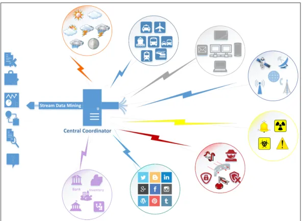
Figure 2.1 Central coordinator monitoring data streams over a sliding window model . 11

Figure 2.2 Miscellaneous data stream application domains . . . 14

Figure 5.1 Minimum requirement ofsupj(XY)for supports ofXandY . . . 35

Figure 5.2 Partial lattice of frequent itemsets with[n−1]rules . . . 36

Figure 5.3 Interesting[n−1],[1−n]and[n−n]association rules with(lif t >1) . . 38

Figure 5.4 Transactions in a bit matrix over sliding window . . . 41

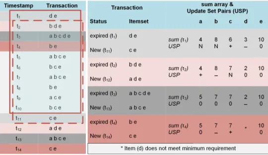
Figure 5.5 Single-pass PAET update: (sliding widow,sumarray,U SP) . . . 45

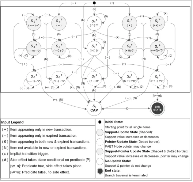
Figure 5.6 States and transitions for incremental update usingHybrid Automaton . . . 47

Figure 5.7 Selection of update settings for state transitions . . . 51

Figure 5.8 Partial lattice of frequent itemsets with[n−1]rules for sliding window (τ2) 54 Figure 5.9 PAET generated from1st sliding window (τ1) of Figure 2.1 . . . 60

Figure 5.10 Comparison of three tree structures: PAET, CET (Moment) and FP-Tree . . 61

Figure 6.1 MAREDS algorithm class diagram . . . 63

Figure 6.2 Association rules and performance evaluation for different datasets . . . 66

Figure 6.3 Performance comparison for T5I4D100K dataset . . . 67

Figure 6.6 Run time and memory usage comparison for BMS-WebView-1 dataset . . . 69

Figure 6.7 Run time and memory usage comparison for BMS-WebView-2 dataset . . . 69

Figure 6.8 Performance comparison over Kosarak dataset . . . 70

(11)

List of Tables

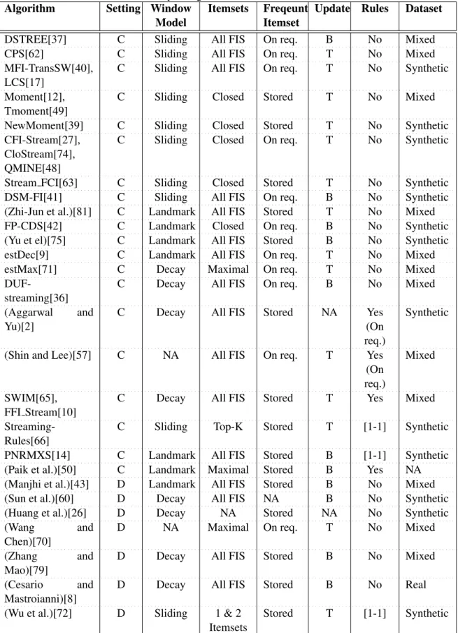
Table 3.1 Survey of algorithms from the literature review . . . 26

Table 5.1 Updating selected rules with the change of support . . . 40

Table 5.2 Hybrid automaton: state accepted input specification . . . 50

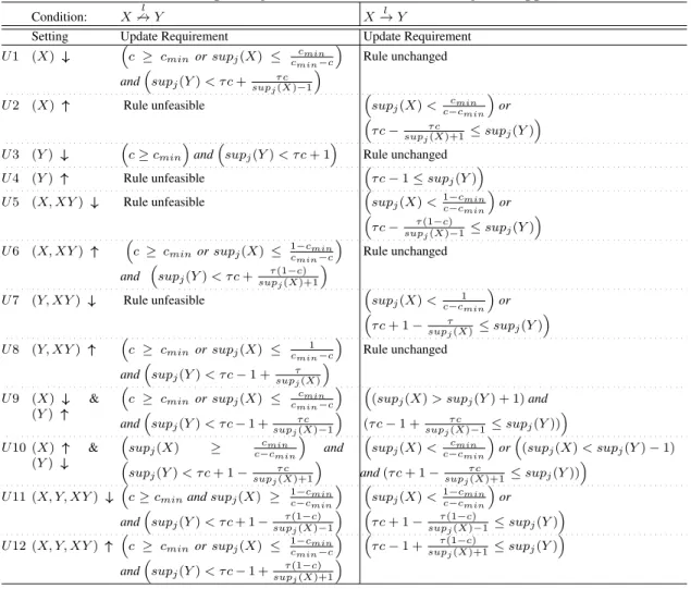
Table 5.3 Requirements for incremental evaluation ofconfidenceandlift . . . 53

Table 5.4 [n − 1] Association rule generation for USP {(a, N),(b, N),(c,+),(d,−),(e,0)} . . . 60

Table 5.5 PAET analysis for various minimum support and minimum confidence values 61 Table 6.1 Experimental datasets characteristics . . . 65

(12)

Chapter 1

Introduction

The rapid technological advancement in the last century has changed our society life style. As computing devices have evolved to become mobile, miniaturized, affordable and human indepen-dent, they have become a vital part of almost every single task of our daily life. The fact that these devices can be equipped with sensing capabilities, strong processing power and advanced communi-cation modules, allows them to form large monitoring networks that generate a huge volume of data continuously at high speeds and in real time. This is referred to as data streams. Such data represent events triggered by changes in environments or live status reports, and therefore they require online processing and analysis in a swift and prompt manner to be able to extract useful information. The huge volume and high arrival rate of stream data makes data storage infeasible. Hence, delays in processing of stream data could cause data and information loss.

Data mining provides several techniques that can explore hidden information within data. How-ever, the characteristics of data streams pose constrains and challenges that traditional data mining algorithms were not designed to take into consideration. In this thesis, we propose a data mining algorithm to mine association rules events from multiple data streams in an incremental manner. The scope of the proposed algorithm lies in identifying frequent associated events that can generate interesting association rules. We investigate a generic and an efficient stream mining approach to produce selective association rules among dependent events from a sliding window over multiple streams. These association rules are determined incrementally in a centralized setting.

(13)

1.1 Motivation

In the recent years, the need to analyze large volumes of data has motivated scholars in the field of data mining to improve the mining processes in order to accommodate large static datasets, mini-mize the resources required in the analysis and generate mining models that represent the data [28]. As the environment hosting or generating the data evolved much more, it was essential for mining processes to address the problem of continuous and rapid data generation. In addition, the telecom-munication technological leaps, in all domains, infrastructure, speed, bandwidth and hardware have encouraged real-time monitoring of different venues of our lives and capturing any possible data for further analysis. Live data is generated in a continuous manner and can be transmitted around the globe rapidly. Some popular examples of data streams include Internet browsing traffic, social media messages, weather information, vehicle guiding systems, road traffic updates and many more. Several businesses and organizations are converting most of their data infrastructure in to a streaming model because of the potential that streams hold and the increasing demand of real-time analysis of data [67]. The challenges of stream mining are increasing as streams are evolving to have faster arrival rates with huge data volume. Recent statistics estimate daily data generated volume to reach 2.5 billion terabytes. This number is expected to grow to 40 billion terabytes by 2020 [16].

Data streams require the design of advanced and efficient algorithms and frameworks that would process, analyze, aggregate different data sources and respond to any query in a real-time fashion while eliminating any unnecessary operations. The generated mining models need to be updated incrementally upon the presence of new data without re-initiating the whole mining process. The mining output needs to be available upon request such that it would represent the current status of the stream data. Consider the following example. A network of sensors deployed to monitor Tsunami incidents and alert authorities of possible warnings or attacks. Different devices continu-ously measure weather conditions, earthquake signs, volcanic eruptions and other parameters [3]. If the generated data was to be stored and analyzed later in an offline manner, disasters will strike without being detected. Therefore, data streams require to be mined promptly and in an efficient and incremental manner.

(14)

to discover interesting relations between data elements in large datasets. Strong association rules are identified using different interestingness measures. Rules can be useful in behavior analysis, situational awareness, event prediction or decision making.

1.2 Objective and Contribution

The concept of ARM was first introduced back in 1993 by Agrawal et al. [3]. Over time, schol-ars presented several similar approaches. Some approaches enhanced the Agrawal et al.’s algorithm, others proposed new approaches. The ARM process is composed of two steps: frequent itemsets are extracted from data and then association rules are generated from these itemsets. In stream data mining, research initiatives mainly focused on the first step. As a matter of fact when mining a data stream with a sliding window topology, majority of the proposed algorithms, discussed in Section 3.1, only attempt to extract frequent itemsets without generating the association rules. Other algo-rithms, Section 3.2, which state that they aim to generate the rules, actually generate the rules on demand without taking into consideration the characteristics of data streams. The objectives of this thesis include analyzing the existing gap in the literature for online rule generation over data streams and proposing a new approach of ARM over data streams. In addition, we perform benchmark association rule generation on existing common datasets and compare performance with existing research work. To the best of our knowledge, this is the first work on incremental association rule mining over a sliding window which extracts and maintains the generated rules. Our contributions in this thesis are summarized as follows:

(1) We introduce a novel algorithm calledMining Association Rules from Event Data Streams (MAREDS)to extract interesting association rules from evolving data streams over a sliding window model in a centralized setting.

(2) We propose an in-memory efficient data structure, thepartial association enumeration tree

(PAET), which maintains frequent itemsets, potential itemsets, itemsets that might become frequent when the window slides, and the relations among the frequent itemsets.

(15)

PAET and incrementally maintain the rules as the data stream window slides.

(4) We implement the proposed algorithm and framework and evaluate the performance over sev-eral real-life and synthetic datasets, in terms of processing time, memory footprint, respon-siveness and scalability. Extensive experiments suggest that the proposed technique performs better than the existing techniques in the majority of the test cases.

1.3 Thesis Organization

The rest of this thesis is organized as follows. Chapter 2 provides background knowledge of frequent itemset mining, association rule mining and stream data mining. Chapter 3 reviews related work. The problem of mining association rules over data streams is defined in Chapter 4. Chapter 5 introduces the proposed incremental association rule mining algorithm over data streams. It presents a case study demonstrating the flow of the proposed algorithm as well. Experimental results are presented in Chapter 6. Chapter 7 draws the conclusion of the thesis and hints at future research directions.

(16)

Chapter 2

Background

2.1 Data Mining

The concept ofdata miningrefers to the process of analyzing large datasets in order to extract hidden knowledge and implicit interesting patterns. Data mining outcomes or models are used in different operations such as decision making, status analysis and prediction of behavior outcomes. The wide range of applications where data mining is useful made it an active researched field. Yet, the term “Data Mining” was not introduced until the early 1990s. The roots of data mining can be traced back to three scientific fields: statistical studies, artificial intelligence and machine learn-ing. The vision and understanding on how to extract useful information from data evolved as these different fields evolved. Early data analysis and pattern identification started via different statistics concepts. In 1775, Bayes and Price introduced Bayes theorem [13, 25], which examined current probability to prior probability. Later, in the early 1800s, regression analysis was introduced [13]. Regression was used to estimate relationships among variables. Then, the computer technologi-cal boom arrived, which increased data collection, storage and manipulation. Data has grown in size, complexity and availability. Data processing has expanded broadly with several advancements in different computer science fields, such as clustering, neural networks, genetic algorithms in the 1950s, decision trees in the 1960s and support vector machines in the 1990s [29, 22]. Today, the demand for data mining is increasing for all domains whether scientific or commercial. Data mining

(17)

techniques have comprehensive analytics and powerful approaches that allow the tackling and anal-ysis of more complex data. End users have access to data mining tools with user-friendly interfaces and graphical mining outcomes.

Data mining involves several techniques, each of which provide different data analysis ap-proaches and output. These techniques can be classified into two categories: descriptive mining andpredictivemining. Descriptive mining approach categorizes or extracts general characteristics or relations of a mined dataset [31]. Association mining, sequential mining and clustering are some of the main tasks involved in the descriptive mining techniques’ tasks. Predictive mining approach analyzes historical data to extract relations or implications in order to predict future data values or part of it [31]. Examples of such are classification, regression and outlier detection. Some of the major data mining techniques are briefly presented below:

• Classification: Classification analysis divides a given dataset into distinguished classes or concepts. Classification models are identified by analyzing a training dataset where the class labels are predefined. These models predict categorical class labels over discrete or unordered datasets with unknown class labels [22].

• Regression: Regression analysis is a statistical approach that divides datasets into classes in a similar manner to classification. Regression uses training datasets to identify distribu-tion trends as well. But unlike classificadistribu-tion models, regression models perform numerical prediction rather than discrete labeling [22].

• Clustering: Cluster analysis shares the same outcome of classification and regression where data is organized into classes. The clustering technique, unlike classification and regression, does not have a defined set of classes. A clustering algorithm discovers proper classes using the principle of “maximizing the intraclass similarity and minimizing the interclass similarity” [22].

• Outlier Analysis: Outliers do not follow the general flow or behavior of the dataset they belong to. Mining algorithms usually label outliers as noise or exceptions. However, in some cases identifying such rare or unusual data can be useful in many fields. For example,

(18)

identifying data packets with unusual payloads can prevent a malware spread or a hacking attack [22].

• Association Analysis: This type studies the frequency of distinct items occurring together in a given dataset and the relation among them. User-defined thresholds, such as itemset minimum support and association rule confidence, are used to limit the mining outcome to interesting results [22, 31]. Association rule mining is described in more details in Section 2.2.

2.2 Association Rule Mining

Association rule mining is one of the descriptive mining techniques that has shown great po-tential and captured scholars attention since it was first introduced in the early 1990s [31]. Its importance rises from its capabilities to discover unapparent relations, interesting correlations, fre-quent patterns, associations or casual structures among data in large datasets. These capabilities create a wide range of applications for association rule mining such as marketing, risk management, inventory control, network management and many more. The association rule mining problem is decomposed into two phases.

Phase I: Mining Frequent Itemsets

Mining frequent itemsets is a major part for several data mining techniques such as association rules, sequential patterns, and classification [61]. Its task is to explore combinations of items with minimum frequency threshold occurring within a dataset. Such combinations are termed as frequent itemsets.

Definition 2.1. (Itemsets). An itemsetX, is a set of items, where(X⊂I)andI ={i1, i2, . . . , in}.

Definition 2.2. (Support). The support of an itemsetXdenotes the frequency ofXwithin a dataset or a sliding window; it may be presented as the ratio of transactions containing all items ofX as well.

(19)

Definition 2.3. (Frequent Itemset). An itemsetX is frequent if itssupport(X) ≥ smin, where

sminis a user-defined threshold for the least acceptable support value, known asminimum support.

Phase II: Association Rule Generation

Association rule generation is defined as forming relationships or correlations among frequent item-sets, extracted in “Phase I”, known as association rules. The generated association rules may not necessarily provide meaningful information. Actually, some of the generated rules are misleading. Several measures are proposed by scholars to measure the interestingness of an association rule. The task of determining the interestingness is not simple nor objective. A rule that may be considered interesting for a particular application, may not be so for another. Two key interestingness mea-sures used in ARM areconfidenceandlift. Both measures have been incorporated into MAREDS functionality. More highlights on association rules, confidence and lift are discussed below:

Definition 2.4. (Association Rule). An association rule is a representation of a relationship between two itemsets in the form of an if/then statement. A rule between itemsetsX, antecedent (if-clause), andY, consequent (then-clause), has the form of(X →Y), where(X∩Y) =φ.

Definition 2.5. (Confidence). The confidence of an association rule refers to the probability of both the antecedent and the consequent appearing in the same transaction. The confidence of association rule,(X→Y), refers to the percentage of transactions containingXthat also containsY.

conf(X→Y) = sup_sup(X₍_X∪Y₎)

For an association rule(X → Y)to be interesting as per the confidence measure,(X∪Y)has to be a frequent itemset andconf(X → Y) ≥ cmin, wherecmin is a user-defined threshold for the

least acceptable confidence value, known asminimum confidence.

Example 2.1. Let us assume we are analyzing a data stream for road traffic. We can note that delay events would often occur with bad weather events. Association analysis might show that70%of the sliding window data that include bad weather events also include delay events. This relationship could be formulated as follows: Bad weather implies delay with70%confidence.

Definition 2.6. (Lift). The lift of a rule indicates the strength of a rule over the random co-occurrence of an antecedent with the consequent, given their individual support. In probability

(20)

theory, lift refers to the joint probability of occurrences for two independent itemsets X and Y. In data mining, lift is treated as a ratio between the confidence of the association rule over the unconditional probability of the consequentY.

lift(X→Y) = _supsup₍_X(₎X_×∪_supY)₍_Y₎

An association rule where the antecedent X and consequent Y are related by a probability that is more than the product of their individual probability of occurrences, or in other words whenlift>1, is considered to be interesting. A lift greater than1indicates thatX andY are dependent and are not occurring randomly together.

Example 2.2. Referring to the previous example of the road traffic data stream for road traffic. Let us assume that the following are support values for some of the events in the sliding window: sup(Accident) = 70%, sup(Delay) = 88%andsup(Accident∪Delay) = 60%. Hence, the rule

conf(Accident→Delay) = 85.71%. Such a rule sounds interesting as it is having high confidence and support values. However, the rulelift(Accident → Delay) = 0.97. In such cases, the over all “Delay” events occurrences are actually less likely to happen as a result of that particular accident.

Several traditional association rule mining algorithms are proposed to mining frequent itemsets and association rules from transactional databases. Agrawal and Srikant [4] have proposed,Apriori, the first algorithm to mine frequent itemsets and generate association rules from a transactional database. Apriori first extracts single-frequent items. The single frequent items are then extended to dual frequent itemsets, itemsets with two items. The process continues until no more itemsets can be extracted. Each round of frequent itemset mining requires a new scan of the dataset. Afterwards, Apriori examines relations within each of the extracted itemsets. A rule is generated by splitting itemsetX into two non-empty sets,Y and(X−Y), represented by(Y → X−Y). A frequent itemsetX, withnitems, generates(2n−2)association rules ignoring those with empty antecedents or consequents(φ → XorX → φ). Rules that do not satisfy the minimum confidence threshold are discarded.

Example 2.3. Let us assume that the extracted frequent itemset isX = {a, b, c}. The itemsetX contains3single items. Hence, the number of generated rules= 23−2 = 6:

(21)

Several variations were proposed to enhance performance of Apriori algorithm. Some of the com-mon variations are bucket-hash itemsets, transaction reduction, candidate itemsets partitioning, data subset mining and dynamic itemset counting [29, 22]. Other new algorithms were proposed as well, such asFP-Growth, where a pre-fix tree is used to represent the database. Non-frequent items are discarded. Each frequent item is mined to extract the frequent itemsets without the need to re-access the database as the tree already holds the needed information [23]. Another proposed al-gorithm mines frequent itemsets using vertical data format where the transaction identifications are grouped by the items. All these variations or new proposals only focus on the first phase of the asso-ciation rule mining, which is frequent itemset extraction. The second phase has not been improved and still has the same complexity which may be acceptable while mining traditional databases. If association rules are to be generated in a stream environment, it may be costly to perform all the second phase operations every time the sliding window is updated.

2.3 Data Streams

A stream of data is defined as a set of consecutive items that arrive in an orderly and timely manner. Streams are usually unbounded and continuous. They arrive at high speed and have dy-namic data distribution. These characteristics of data streams make them distinct from traditional static data stored in databases or data warehouses. Therefore, new data analysis tools are needed to tackle data streams accordingly [28].

Streams consisting of distinct events in a general form are often described asmoments in the research literature [55]. Moments are useful in understanding distribution of items’ frequencies, analyzing stream properties and storing stream related knowledge in an optimized manner [55]. Stream data is presented as a set of co-occurring events which can be seen as an itemset where each item represents an event. Thus, a data stream denotes a temporal sequence of itemsets, also known as astream transaction. Figure 2.1 depicts a sequence of data stream transactions. For example,

(22)

Figure 2.1: Central coordinator monitoring data streams over a sliding window model

2.3.1 Data Stream History

Even though the interest in stream data is relatively recent, the concept of streams goes back for more than half a century. The term “Stream” was first introduced by Landin, in 1966, to model histories of loop variables when designing unimplemented computing languages [33]. In the next years, the concept of stream has been mainly discussed within the literature of data flow field [64]. Today, stream data analysis and mining have become an active area of research in computer science.

(23)

2.3.2 Applications

In this section we discuss some of the real-life data stream application domains in which data mining plays an important role. The data mining in streams helps to flag out unwanted or unique sit-uations from normal behavior, extract patterns, identify adversary actions or customize information [1]. Figure 2.2 illustrates different data stream domains.

• Networks and Telecommunications: Network traffic forms one of the largest streams which holds tons of information. Analysis and mining of such streams helps in cyber-attack preven-tion, prevention of private data accessibility, detection of suspicious behaviors or intrusions, analysis of networks and user online-behavior and many more [20, 58].

• Financial and Stock Markets: Financial transaction streams are used to detect possible inter-net banking and credit card frauds. It is used in bankruptcy prediction for loan takers as well. In stock markets it is used to prevent and detect possible insider trading [18, 20, 52].

• Roads and Transportation: Streams from monitored roads and highways provide us with several useful information such as traffic forecast, expected travel times, suggested routes and alternative routes for navigation systems [7, 46].

• Medical Care:Some patients are provided with sensors to monitor their health conditions and vital signs. The data stream generated from aggregating the sensors output helps in detecting possible medication reaction, organ failures and internal injuries [1].

• Social Media: In the era of social media, social information such as posts, tweets, followers, followed by, likes and shares, generate one of the largest available data streams. Analysis and mining of social streams is used to identify the users’ or entities’ interests and preferences, predict their behaviors and habits and provide them with personalized services and products [21].

2.3.3 Types and Models

Data streams are categorized into two types according to the nature of the data perceived in the stream,offlineandonline[64].

(24)

Definition 2.7. (Offline streams.) Offline streams are bulk data that occur at regular time intervals. However, the flow of data is not constant. Data updates arrive at fixed times, daily, weekly, or monthly, with periods of inactivity in between.

Definition 2.8. (Online streams). Online streams refer to real-time data that arrive in an orderly manner.

Analysis and queries on data from offline streams are done in an offline manner and in respect of all previously received saved data [64]. Updating tasks in data warehouses are good examples of this type. Meanwhile, in online streams the data arrival rate and data volume are both high, causing the data storage to be infeasible. Online data streams usually represent a live situation which may require prompt analysis to extract useful live information. Internet-packets represent an online stream, which is impossible to store, yet needs to be analyzed promptly to anticipate any possible attacks.

Furthermore, when addressing data streams in a data analysis context, streams are categorized into three models based on which part of the data stream is used in the analysis or the mining process. Below are the description of each model:

Definition 2.9. (Landmark Model). In the landmark model the mining process includes all the stream data starting from a defined point of time, known as theLandmark, till the present. The outcome for such a model is practical for applications interested in historical data [54, 53].

Definition 2.10. (Damped - Time Fading Model). In the damped model a weight is assigned to each transaction in the stream. The weight value is inversely correlated with the transaction’s age. This impacts old transactions to have less effect on the analysis or mining process outcome. Such a model is suitable for applications that require to consider historical data in the analysis process, yet the emphasis should be on newly available data [54, 53].

Definition 2.11. (Sliding Window Model). The sliding window model maintains the most recent stream transactions in a buffer, called a window. The window has a fixed size that may vary accord-ing to the application and/or system resources. When new transactions arrive, the oldest transactions are removed from the window. The same concept applies to any analysis or mining process. Anal-ysis or mining is only applied on the transactions in the current window. Once new transactions

(25)

are available and old ones are retired, the outcome is updated accordingly. Outcome of this model is desirable for applications seeking recent information from data streams [54, 53]. This process is known as a forgetting process, as it limits the amount of processed data and allows the mining process to forget old data and adapt to changes [7].

Usually the offline streams use a landmark model in the data analysis process, while online stream use either the damped model or the sliding window model as the outcome is expected to reflect the live information from the stream.

Figure 2.2: Miscellaneous data stream application domains

2.3.4 Challenges and Requirements

The stream data environments, unlike conventional databases and data warehouses, impose a set of challenges that make traditional analysis and mining algorithms fail or perform properly. The following elaborates on the major challenges and requirements of data stream analysis and mining algorithms [28, 30, 64, 1, 20].

(26)

• Unbounded Data Feed:Traditional data mining techniques analyze data in an offline fashion, where the data is stored in databases which offers the mining algorithm the luxury of multiple accesses. However, data streams are generated in an unbounded manner which makes storing all the data infeasible. Old data needs to be discarded to free space for newly arriving data. Hence, a stream mining algorithm is required to perform the mining task after a single data scan only.

• Real-Time Mining: A key characteristic of a stream is that the data’s arrival is rapid. The mining algorithm has to process the data in a real-time manner while taking into consideration the datas arrival rate. A relaxed processing time can cause a bottleneck or even data loss as the data arrival rate is faster than the processing rate.

• Resource Management: A traditional mining algorithm is considered to be finite. It per-forms its assigned mining task and eventually terminates. On the contrary, a stream mining algorithm runs continuously and does not pause or end unless manually terminated. It con-stantly requires some of the systems resources from processing power, memory space and sometimes power energy. A stream mining algorithm requires proper resource management such that it would not exhaust the systems resources or block other processes from having them. Advanced scheduling and memory management techniques are important to take into consideration when designing a stream mining algorithm.

• Data Structure Choice:The choice of a proper data structure is an important element in any algorithm design. It is even more important for stream mining. Data structures are used to store the stream data and the mining outcome. In addition, data structures are accessed to update both incoming data and the mining outcome, or to retrieve information in response to users’ queries. Hence, a stream mining algorithm needs to choose an efficient and a compact data structure that has a small memory footprint where data can be accessed with as mini-mum operations as possible. Storing any data on the disk has an additional overhead of I/O operations increasing the processing and data access time.

(27)

mentioned in the previous point, several challenges rise regarding the extracted knowledge. Newly discovered knowledge has to be added or merged with the previous knowledge in an incremental manner. In addition, old knowledge has to be either degraded or retired.

• Visualization: Visualization is a powerful tool to understand and illustrate the data mining outcome. In some data stream applications, such as monitoring applications, visualization facilitates the analysis process. For example, a use of a graph that shows the relationship between mined association rules makes any action taking or decision making process easier and faster.

• Data Evolution: Stream data is generated in a rapid manner and represents real-world appli-cations and environments. As the conditions change or differ in the environments, the under-lying distribution of a data stream changes over time. This change may require a change in the user defined parameters, such as the minimum support or minimum confidence. A well designed stream mining algorithm should have some flexibility to interact with such require-ment without the need to start the mining process all over again.

2.3.5 Challenges of Mining Data Streams

Data streams require real-time mining, which refers to mining the data as soon as it is generated and available. Traditional data mining techniques mine data in an offline fashion, where the data is stored and the algorithm has easy and multiple accesses to it. However, as stream data is generated in a huge, rapid and timely manner, storing all the data is infeasible. A stream mining algorithm has to extract information from generated data using only one data scan while taking into consideration the data’s arrival rate. Additional mining operations, such as a second data scan, is resource consuming and can cause a bottleneck as data may arrive faster than the processing rate [54].

2.3.6 Concept Drift

The distribution of the generated data in a stream may change over time. This concept is known as temporal evolution, covariate shift, non-stationarity, or concept drift [7]. Concept drift occurs from unforeseen or unpredictable changes that may affect the sources generating stream data. The

(28)

distribution of data in traditional databases is assumed to be static. However, this is not the case for real-time stream applications. The data in streams is being generated continuously. Hence, it is typical that different parameters and conditions reflected by such data to change over time. The distribution of data will change eventually as well. Traditional data mining models and algorithms may have poor performance or may produce inaccurate information if applied on stream data. A stream mining algorithm should be able to capture the change in data distribution and reflect it in the mining outcome. Concept drift in data streams urged to introduce new concepts such as the sliding window model, which was discussed earlier in Section 2.3.3.

(29)

Chapter 3

Literature Review

The motivation of this thesis is to build a generic, fast and scalable data stream mining technique to extract associations among events during decision making in various application areas. In this regard, a prescriptive data mining technique like ARM has shown great potential and captured scholars’ attention since it was introduced in the early 1990s [32]. The fist frequent itemset mining over data streams was proposed by Manku and Motwani in 2002 [44]. The authors proposed an algorithm to mine single frequent items from a data stream. Later, they extended their scope to mine frequent itemsets. And since then several algorithms were introduced to tackle ARM over streams. Data stream mining algorithms are often categorized by two dimensions:

• Centralized versus Distributed: In a centralized setting, items are collected from various streams in a central location, known as a sink or coordinator, where the mining process takes place. In a distributed setting, data streams are mined at distinct locations. Each individual mining output is aggregated to form one global mining outcome.

• Frequent Itemset Mining versus Association Rule Mining: Frequent itemset mining extracts itemsets that meet a minimum support threshold in a dataset. As mentioned earlier, this is considered as the first phase of the two-phase ARM technique. In its second phase, association rules are formed from the extracted frequent itemsets of the first phase. Rules are filtered afterwards as per user or application requirements.

(30)

important. Without the rule extraction, the information gained in the first phase may be misleading and can not be used directly in decision making. Hereafter, we review relevant related literature in data stream association rule mining categorized as stated above.

3.1 Centralized-Stream Frequent Itemset Mining

In the sliding window model, we focus on algorithms that mine whole and closed frequent itemsets with exact outcome as it is more relevant to our proposed algorithm, MAREDS. Algorithms that mine maximal itemsets or provide approximate outcome is information lossy. They may also have marginal errors or produce some false positive or false negative results. Hence, such algorithms are not considered.

Leung and Khan [37] propose one of the first algorithms to mine exact frequent itemsets from a data stream. The algorithm adopts a batch processing model with non-overlapping sliding win-dows. Incoming data is stored in a canonical ordered prefix-tree structure,DSTree. The tree nodes store current items support values and some particulars from the previous batch. Previous batch information is used to prevent any tree traversal during the update process. FP-growth mining tech-nique [23] is used to extract the frequent itemsets from the DSTree. Tanbeer et al. [62] also use FP-growth mining technique but over a transactional based sliding window. The window trans-actions are maintained in an FP-tree-like structure, known asCPS-tree. CPS-tree is restructured occasionally to keep the nodes in descending order based on their support values. The restructuring process provides rapid tree accessibility and keeps its size minimal. Li and Lee [40] introduce MFI-TransSWalgorithm which uses a bit sequence data structure to store the sliding window items. Left bit-shifting is used to add new transactions and retire the old ones while the AND operation is used to extract the frequent itemsets. LDSalgorithm by Deypir and Sadreddini [17] uses three different forms of lists to store the sliding window items. The first list maintains items by the transactions they are present in. The second list maintains items through the transactions they are absent from. In the third list, item occurrences are stored as a bit string. Each item is maintained in the most optimum list type based on its frequency. Frequent itemsets are extracted from the lists upon user request using either Eclat[76], dEclat[77] or bEclat[6] algorithms. The choice of algorithm depends

(31)

on the most common list type.

Chi et al. [12] proposeMomentalgorithm, the first algorithm to mine closed frequent itemsets over a data stream using a sliding window. Moment stores window transactions and extracts closed frequent itemsets in an inverse FP-Tree and a prefix tree structure, namedCET, respectively. CET maintains additional nodes, known as boundary nodes, to address state changes such as: infrequent itemset becoming frequent and vice versa. The proposed concept of boundary nodes is so intuitive, yet it has a major flow. The number of maintained boundary nodes is relatively high compared to the number of closed frequent itemsets nodes especially with low minimum support value. This would cause slow tree traversal and memory exhaustion. NewMomentby Li et al. [39] andTMomentby Nori et al. [49] propose variations of the Moment algorithm. The sliding window transactions and the mined closed frequent itemsets are maintained in a prefix tree in both algorithms. In addition, a copy of the closed frequent itemsets are stored in a separate hash table to ease any update or query task. The first level nodes in the tree are used to store all items along with their occurrence information. This information is used to track the items’ supports and extract the frequent itemsets. NewMoment represents the occurrences using a bit string while TMoment uses an integer array of transaction unique IDs. The other tree nodes hold the closed frequent itemsets and their support. Jiang and Gruenwald [27] proposeCFI-Streamthat stores all the sliding window transactions, fre-quent and infrefre-quent, in a prefix tree in a closed itemsets format. Frefre-quent itemsets are extracted upon user request by applying minimum support threshold. CloStreamby Yen et al. [74] maintain all the sliding window transactions as well. CloStream creates two tables to store current transac-tions and single items separately along with a list of closed itemsets. QMINEalgorithm [48] also uses two similar tables. However, the second table in QMINE holds a set of bit victors to keep track of each item’s presence in the first table. Both CloStream and QMINE algorithms generate frequent itemsets upon request and by applying desired minimum support value. Keming Tang et al. [63] propose Stream FCI which uses an FP-tree like structure, calledDFP-tree, to store the sliding window transactions. Frequent items and their support are stored in an external head table. Each frequent item points to its first occurrence in the tree. In addition, the algorithm creates links across matching items in different tree branches. The extracted closed frequent itemsets are saved in a separate table to ease update and query operations.

(32)

The landmark model analyzes all data in a stream starting from a defined point of time. Data volume grows to infinity as time goes on. Some data needs to be discarded and hence the mining outcome will not represent exact frequent itemsets. In this model, Li et al. [41] proposeDSM-FI

algorithm to mine frequent itemsets from a data stream by batch. Batch data is stored in a prefix-tree. Tree pruning is applied periodically to remove infrequent or irrelevant itemsets and keep the tree size minimal. Frequent itemsets are extracted from the tree periodically or upon request. Zhi-Jun et al. [81] propose dividing frequent itemsets into equivalent classes. Each class itemsets, support values and border itemsets are maintained in an enumeration tree. The border itemsets are used to filter frequent itemsets and hence keep tree size under control. Liu et al. [42] propose FP-CDS

algorithm to mine closed frequent itemsets over the same model. Potential frequent itemsets in each batch are stored in a prefix tree. Frequent itemsets are extracted from the tree in real time upon user request. Yu et al. [75] propose a false-negative based algorithm to extract approximate frequent itemsets.Chernoff Bound[11] is used to prune off infrequent itemsets as more data arrive.

Over a stream damped model, Chang and Lee propose estDecalgorithm [9] to mine frequent itemsets. estDec maintains itemsets that have potential to become frequent in the near future in a lexicographic tree. Decay element is represented by a weight value assigned to each of the nodes in a reverse chronological order. Frequent itemsets are extracted from the tree upon user request. Woo and Lee [71] extend estDec toestMaxalgorithm to mine maximal frequent itemsets. In estMax, after adding potential itemsets to the lexicographic tree, the tree is restructured to keep only maximal frequent itemsets. estMax uses two thresholds,Maximality MarkandMaximum Lifetime, to improve mining performance. The Maximality Mark identifies new nodes and eliminates the need to fully traverse the tree upon update. Maximum lifetime is used to opt out old frequent itemsets. Leung and Jiang [36] propose DUF-streaming algorithm to mine frequent items over a damped model by batches. DUF-streams usesUF-growth algorithm [35] to extract frequent itemsets and stores them in an FP-like tree. An “Expected Support” value, representing the decay element, is computed incrementally after processing each batch to eliminate older itemsets.

(33)

3.2 Centralized-Stream Association Rule Mining

Aggarwal and Yu [2] are among the first scholars to propose a framework for online mining of frequent itemsets and generating association rules. The proposed concept of online mining provides end users with capabilities of directly querying a database of generated association rules. Queries have the flexibility of using different support and confidence values without any additional com-putational cost. An adjacency lattice is used to maintain extracted frequent itemsets. The lattice structure allows easy association rules generation, as well as rule redundancy removal. It eliminates the need to re-access original data for support queries. The algorithm does not take into consid-eration any dataset update or any transaction insertion and deletion, which makes it not suitable for data streams. Shin and Lee [57] propose an algorithm to mine association rules over a damped stream model. Frequent itemsets are mined usingestDecalgorithm [9]. Afterwards, a stack traver-sal approach is used to generate association rules. The generation process divides rules into ordered rules and unordered rules. Ordered rules indicate that all items on the left-hand side are lexico-graphically greater than those on the right-hand side. However, the algorithm does not keep track of generated rules. It requires to generate rules from scratch upon each user request by traversing the estDec tree. Thakkar et al. [65] propose a data stream management system which mines association rules over a sliding window model. Frequent itemsets are mined usingVerificationalgorithm [47] and maintained in an FP-like tree. Association rules are generated after a predefined number of elapsed transactions. Optional pruning is applied over the extracted rules to eliminate duplicate and uninteresting rules. Association rules are saved in a database for further analysis and rule compar-ison. However, the saved rules are not used in subsequent rounds of rule generation. Su et al.[10] proposeFFI Streamto mine association rules from stream data containing quantitative attributes. Stream data is divided into fuzzy sets usingSWEM clustering algorithm [15]. Afterwards, frequent itemsets are acquired from the sets using modified version ofUF streaming[35]. A “Membership Function Bias”, known asMFB measure, is proposed to measure interesting frequent itemsets that could generate interesting association rules. Yet, rules are not actually generated. Thool and Voditel [66] proposeStreaming-Rulesalgorithm to mine association rules over a landmark window model. Frequent itemsets are mined usingSpace-Savingalgorithm [45] and maintained in a list structure.

(34)

One-to-one association rules are generated by rescanning the current window. The rule generation process is not incremental. It is done from scratch upon every data update. Corpinar and Gundem [14] proposePNRMXSalgorithm to mine positive and negative association rules fromXMLstreams over a landmark model. A modified version of FP-growth [23] is used to mine frequent itemsets from each stream batch. The rule generation process extracts one-to-one association rules from scratch in a non-incremental way. Paik et al. [50] propose to mine maximal frequent items from

XMLstreams. Association rules are generated for each batch separately. Then, they are filtered by a minimum confidence threshold. Association rules from each batch are accumulated for the entire stream in a landmark model fashion. Yet, the rule extraction for each batch is performed from scratch every time. Vijayarani and Prasannalakshmi [68] conduct an analysis on association rule generation over data streams using traditional mining approaches. The objective of the experiments was to examine the number of extracted rules and the execution time with various data arrival rates. The experiments adopt a batch mining approach. The mining task starts from scratch for each batch. Such behavior does not reflect stream mining environment.

3.3 Distributed-Stream Association Rule Mining and Frequent

Item-set Mining

Park and Kargupta [51], Sawant and Shah[56] and Zeng et al. [78] conduct surveys that in-vestigate approaches for distributed data mining. Majority of surveyed algorithms assume that the datasets are stored in distributed locations across the network. In addition, they deem to have the luxuries of traditional data mining techniques mentioned earlier. These algorithms mainly focus on frequent itemset mining and do not examine any mechanism for rule generation. Moreover, only few articles can be seen on distributed ARM over stream data.

Manjhi et al. [43] propose to extract frequent items from multiple distributed streams. Distinct monitors maintain single items support for each stream. Frequent items are communicated peri-odically to a central monitor in a hierarchical manner. A local monitor communicates its frequent items to an upper level monitor, which merges it with its own items and pass it to the next level. This process goes on until the all frequent items are gathered at the central monitor. The hierarchical

(35)

architecture minimizes communication and computation cost at the central monitor. In addition, it allows more frequent items to be extracted minimizing the error. Sun et al. [60] propose a frame-work to extract frequent patterns from several distributed data streams. Frequent patterns are mined from each stream using adaptive filtering techniques. Global patterns are extracted after aggregating local patterns. Then, they are communicated back to local streams to refine and verify the newly extracted outcome. Huang et al. [26] propose a distributed sequential pattern mining algorithm that uses twoMap-Reducefunctions over aHadoopplatform [5]. The first function extracts can-didate patterns locally at different Hadoop nodes and generates a summary. The second function aggregates the generated different summaries to produce a final summary. The global summary is updated incrementally to incorporate new candidates and remove expired ones. Wang and Chen [70] propose a frequent itemset mining framework over distributed data streams using a landmark model. hSynopsis algorithm [69] is used to mine local frequent itemsets. A central coordinator aggregates local streams synopsises to form a global synopsis. The framework poses communica-tion strategies and constraints that minimize communicacommunica-tion with the coordinator. Zhang and Mao [79] use a combination of decision trees andna¨ıve Bayesclassifier [34] to mine frequent patterns from distributed data streams. Local streams build decision trees to generate statistical summaries. A statistical summary approximates items’ support values of the current stream batch. Then, local patterns are formed from both statistical summaries and key attributes in the decision tree. The na¨ıve Bayes classifier is used to aggregate local patterns to form global patterns. Cesario and Mastroianni [8] propose a hybrid single-pass/multiple-pass framework for mining frequent items and itemsets from distributed data streams. The framework consists of multiple layers of mining. The mining outcome is communicated forward and backward, locally and globally, across the different layers to refine the mining output and minimize the error. Finally, Wu et al. [72] propose a decentralized approach to mine event association rules over multiple streams. Frequent stream events are filtered locally and communicated to a central location where they are merged through an Apriori-based map-reduce function. Association rules are generated through another map-reduce function upon user request. Generated rules are not stored nor are used in subsequent requests.

Table 3.1 presents an overview of related work discussed above. As elaborated, scholars in centralized setting focus on frequent itemset mining. Association rule generation is not discussed

(36)

thoroughly in data streams. Available stream rule-generating algorithms mainly extract all frequent itemsets and then apply traditional techniques to extract the rules. They do not take into consider-ation any stream characteristics. This leads to several unnecessary computconsider-ations that are so costly in a stream environment. In distributed setting, most of the techniques require reliable and exten-sive communication of information to share the information. The techniques do not consider any information that would be lost because of the lack of a global data view. In the proposed algorithm, MAREDS maintains interesting associations incrementally from data streams without the need for any further computations.

(37)

Table 3.1: Survey of algorithms from the literature review

Algorithm Setting Window

Model

Itemsets Freqeunt Itemset

Update Rules Dataset

DSTREE[37] C Sliding All FIS On req. B No Mixed

CPS[62] C Sliding All FIS On req. T No Mixed

MFI-TransSW[40], LCS[17]

C Sliding All FIS On req. T No Synthetic

Moment[12], Tmoment[49]

C Sliding Closed Stored T No Mixed

NewMoment[39] C Sliding Closed Stored T No Synthetic

CFI-Stream[27], CloStream[74], QMINE[48]

C Sliding Closed On req. T No Synthetic

Stream FCI[63] C Sliding Closed Stored T No Synthetic

DSM-FI[41] C Sliding All FIS On req. B No Synthetic

(Zhi-Jun et al.)[81] C Landmark All FIS Stored T No Mixed

FP-CDS[42] C Landmark Closed On req. B No Synthetic

(Yu et el)[75] C Landmark All FIS Stored B No Synthetic

estDec[9] C Landmark All FIS On req. T No Mixed

estMax[71] C Decay Maximal On req. T No Mixed

DUF-streaming[36]

C Decay All FIS On req. B No Mixed

(Aggarwal and

Yu)[2]

C Decay All FIS Stored NA Yes

(On req.)

Synthetic

(Shin and Lee)[57] C NA All FIS On req. T Yes

(On req.)

Mixed

SWIM[65], FFI Stream[10]

C Decay All FIS Stored T Yes Mixed

Streaming-Rules[66]

C Sliding Top-K Stored T [1-1] Synthetic

PNRMXS[14] C Landmark All FIS Stored B [1-1] Synthetic

(Paik et al.)[50] C Landmark Maximal Stored B Yes NA

(Manjhi et al.)[43] D Landmark All FIS Stored B No Mixed

(Sun et al.)[60] D Decay All FIS NA B No Synthetic

(Huang et al.)[26] D Decay NA Stored NA No Synthetic

(Wang and

Chen)[70]

D NA Maximal On req. T No Mixed

(Zhang and

Mao)[79]

D Decay All FIS Stored B No Mixed

(Cesario and

Mastroianni)[8]

D Decay All FIS Stored B No Real

(Wu et al.)[72] D Sliding 1 & 2

Itemsets

Stored T [1-1] Synthetic

(38)

Chapter 4

Problem Description

In this chapter, we formally define the association rule mining problem over data streams. In Section 4.1, we review the foundations of association rule mining in a data stream environment. The problem statement is stated in Section 4.2.

4.1 Initial Definitions

In a centralized setting, we assume the set of all possible items, also referred as theAlphabet, generated by a data stream is represented byA = {e1, e2, . . . , en}. A coordinator would receive

co-occurring events as a set of items at each defined moment or timestamp tj. The set of items

arriving at the same time stamptj form one itemset and is referred to as a transaction. Relations

between items with itemsets are examined to identify association rules.

Definition 4.1. (Strong Association Rule). The relationship among two mutually exclusive itemsets XandY (X, Y ⊂ A) is deemed to be strong if it follows two conditions. First, the support value of (X∪Y)should be at leastsminwithin a predefined number of recent transactionsτup to the current

moment. Second, the ratio of(X∪Y)’s support compared toX’s support should be at leastcmin

within the lastτ transactions. Such relation betweenX andY is defined as astrong association ruleand is denoted by(X→Y). In data miningXandY are called as antecedent and consequent respectively.

(39)

minimum confidence, respectively. In MAREDS, we investigate an additional condition. We are interested in association rules where antecedentX and consequentY are related by a probability more than the product of their individual occurrence’s probability, hence the association rule lift should be greater than one. The notion of lift was discussed in Section 2.2. We denote association rules that satisfy these three conditions asinteresting rules.

Definition 4.2. (Interesting Association Rule). An interesting association rule is a strong association rule that has lift value greater than 1.

As the window slides, a new transaction is added to the window while the oldest transaction is removed. All the relationships among itemsets require to be re-investigated as some of the itemsets’ support values may change. Wu et al. [73] defines the support and confidence values of an itemset over a timestamped data stream using alifetimefunctionlj.

Definition 4.3. (Lifetime function). At a momenttj, a lifetime functionlj is defined over a sliding

window of sizeτ aslj :A →T.T is a set of timestamps expressed as:{t:j−τ < t≤j;t∈T}.

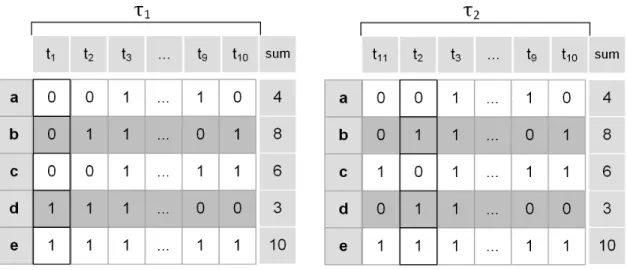
Example 4.1. In Figure 2.1, let us assume that the sliding window sizeτ = 10. Then,l10(a) = {t3, t5, t7, t9}andl10(ab) ={t3, t5, t7}.

The association rules are examined in the same manner as they are dependent on support and confi-dence values. In this context, we introducemomentary association rule.

Definition 4.4. (Momentary Association RuleRj). The associationRjis examined among two sets

of itemsX andY in the most recentτ transactions ending at timestamptj of the sliding Window.

Rj is characterized through three functions: momentary support (supj), momentary confidence

(conf_j) and momentary lift (lift_j) of itemsetXas follows:

supj(X) =| ⋂ e∈X lj(e)|;X ⊆ A (1) conf_j(X→Y) = supj(X∪Y) supj(X) ;X, Y ⊆ A (2) lift_j(X →Y) = τ ×supj(X∪Y) supj(X)×supj(Y) ;X, Y ⊆ A (3)

(40)

From equation (1), it is observed thatsupj(X)≥supj(X∪Y). This is also known as theApriori

property [32]. Similarly, from equation (2), the confidence is also related asconf_j(X → Y) ≥ conf_j(X→Y ∪Z)andconf_j(X →Y)≤confj(X∪Z→Y \Z)whereZ ⊂Y.

Based on the above functions, we define the following related terms:

Definition 4.5. (Stream Frequent Itemset). An itemset X with momentary support no less than smin, i.e.,supj(X)≥smin, is consideredfrequent. Otherwise, the itemsetXisinfrequent.

Definition 4.6. (Omnipresent Itemset). An itemsetXthat is present in all the window transactions, i.e.,supj(X) =τ, is consideredomnipresent.

Definition 4.7. (Intermediate and Closed Itemsets). If a frequent itemsetXhas a supersetX∪Y that has the exact same support ofX and there is no superset ofX∪Y that has the same support, thenXandX∪Y are calledintermediate itemsetsandclosed itemset, respectively. For simplicity, X∪Y is represented asXY in the rest of this thesis.

Association rules can be categorized based on the number of items in the antecedent and the consequent as follows:

(i) [1−1]: named one-to-one rule. It refers to association rules where only single items are present in each of antecedent and the consequent.

(iii) [n−1]: named many-to-one rule. It refers to association rules where multiple items are present in the antecedent, while the consequent holds only single items.

(ii) [1−n]: named one-to-many rule. It refers to association rules where only a single item is present in the antecedent, while the consequent holds multiple items.

(iv) [n−n]: named many-to-many rule. It refers to association rules where multiple items are present in both of antecedent and the consequent.

4.2 Problem Statement

In a centralized setting, a coordinator collects event data streams generated from various mon-itored environments. The problem is to extract and maintain[n−n]momentary association rules

(41)

R_j of our interest from the most recentτ transactions ending attjfrom the data stream. The

inter-esting association ruleRj is incrementally generated using previously stored outcome information

during the mining ofRj−1. An interesting association rule is denoted as(X −→l Y)and satisfies the

following constraints:

(i) supj(X∪Y)≥smin

(ii) conf_j(X →Y)≥cmin

(iii) lift_j(X →Y)>1

* X, Y ⊂ AandX∩Y =φ.

Figure 2.1 is an example of a central coordinator analyzing an event data stream with alphabet

A={a, b, c, d, e}over a sliding window of sizeτ = 10. We use this example throughout the thesis with minimum supportsmin= 3and minimum confidencecmin = 0.7.

(42)

Chapter 5

Proposed Algorithm

Rajaraman and Ullman [55] point out that the core challenge of stream mining lies in handling the rapid speed of the data stream with the complexity of the mining algorithm(s). They recom-mend in-memory, single-pass and real-time data processing. We propose, MAREDS, an in-memory mining algorithm of a selected set of association rules in a centralized data stream setting. The mining procedure captures stream data using a bit matrix and a prefix tree, the partial association enumeration tree, over a sliding window model. The proposed approach enables us to answer the query “What are the current interesting associations rules? ” at any time.

In the next Section 5.1, we analyze different association rule generation properties that would help in reducing the solution space.

5.1 Association Rule Property Analysis

The associations among itemsets in the sliding window may change their status from relevant to irrelevant, and vice versa, upon the arrival of each new transaction. This happens due to changes in the items’ support values and their co-occurrence with other events. In this regard, we examine a set of properties that would help in reducing the solution search space and thereby improve the efficiency of the association rule generation algorithm. We extract the following properties from the aforementioned constraints stated in the problem statement Section 4.2:

(43)

rules are: conf_j(abc → d) ≥ confj(ab → cd) ≥ confj(a → bcd). Hence, the confidence

values of association rules generated from the same itemset have an anti-monotonic property. The confidence functionconf_j is anti-monotonic with respect to the number of items in the antecedent. Ifconf_j(abc→d)does not hold, there exists no association rules among the items in{abcd}at the higher order[n−2],[n−3], etc, where the consequent is a superset ofd. This significantly reduces the scope of the rule search. Property 1 mathematically captures our interest.

Property 1. Given frequent itemsetsX,XY,XZandXY Zare related through an anti-monotonic relationship such that if(X→Y)or (X→Z)or(XY →Z)or(XZ →Y)then(X→Y Z).

Proof. In order for association rule(X→Y Z)to fulfill constraint (ii): [supj(XY Z)

supj(X) ≥cmin],

then using Apriori property:

supp_j(XY)

supp_j(X) ≥ cmin,

supp_j(XZ)

supp_j(X) ≥ cmin,

supp_j(XY Z)

supp_j(XY) ≥ cmin and

supp_j(XY Z)

supp_j(XZ) ≥ cmin.

Any itemset that is present in every transaction of the current sliding window cannot generate in-teresting association rules. For example, a special weather condition may persist for a whole day. Property 2 helps in pruning the scope of search for interesting association rules among frequent itemsets. It signifies that omnipresent data is not relevant to be included in the interesting associa-tions among two set of recent events.

Property 2. An interesting association rule can not have an antecedent and/or consequent itemset that is omnipresent; otherwise, the lift value is less or equal to 1 (lift≤1).

Proof. Assume(X→Y)is an association rule where itemsetXis present in all transactions.

lift_j(X → Y) = τ×supj(XY)

supj(X)×supj(Y) andsupj(x) = τ, thenliftj(X → Y) =

supj(XY)

supj(Y) ; and since

supj(XY)≤supj(Y), thenliftj(X →Y)≤1. The same can applied if itemsetY is omnipresent.

An intermediate itemset X which is subset of a closed frequent itemset XY indicates that these itemsets occur together. Therefore, as stated in Property 3, the relationship between such itemsets will form an interesting association rule, unless they are omnipresent. The generated rule, (X−→l Y), does not require any confidence or lift evaluation .

(44)

Property 3. Given a frequent closed itemset XY and an intermediate itemset X, there exists an interesting association rule(X−→l Y)if itemsetY is not omnipresent.

Proof. Since,supj(X) =supj(XY):

-X,Y andXY are all frequent (Apriori property), constraint (i) is met. -conf_j(X→Y) = supj(XY)

supj(Y) = 100%, constraint (ii) is met.

-lift_j(X → Y) = _supτ

j(Y). So, ifY is not omnipresent(supj(Y) < τ), thenliftj(X → Y) > 1,

which meets constraint (iii).

The following properties, Property 4, Property 5 and Property 6, extend the general concept of Property 3. They provide various conditions to mine interesting association rules. Our main in-terest in this context is to make use of co-occurring events through these properties to improve the performance of the incremental association rule mining algorithm by reducing the search space.

Property 4. Given a non-omnipresent frequent closed itemsetXY Zand intermediate itemsetsX, XY , then(X −→l Y Z),(XY −→l Z),(XZ →−l Y),(X−→l Y)and(X−→l Z)are all valid interesting association rules except in the case(s) where the consequent(s) are omnipresent.

Proof. Using both Property 1 and Property 3.

Property 5. Given a frequent itemsetX, an intermediate itemsetXY and a non-omnipresent fre-quent closed itemsetXY Zsuch thatsupj(XY) =supj(XY Z), the following is true:

a. if(X −→l Y)⇒(X−→l Y Z) b. if(X −−→l Y Z)⇒(X l − − →Y)

Proof. Proof as follows:

a. Given(X−→l Y)is an interesting association rule, it meets constraints (i), (ii) and (iii). - Sincesupj(XY) = supj(XY Z)then implication (X → Y Z) meets constraints (i) and

(ii).

- Sincesupj(Y) ≥ supj(Y Z), then τ

×supj(XY)

supj(X)×supj(Y) ≤

τ×supj(XY Z)

supj(X)×supj(Y Z). Thus, the